Introduction to Arbitrage Pricing Theory (APT)

From a Single Factor to Multiple Factors

The central critique of CAPM is its reliance on a single factor. It assumes that the only systematic risk that matters is an asset's sensitivity to the overall market. However, common sense and empirical observation suggest that different assets are sensitive to different economic forces. For example:

• An airline's stock might be highly sensitive to changes in oil prices.
• A multinational corporation's stock might be heavily influenced by exchange rate fluctuations.
• A utility company's stock might be more sensitive to changes in interest rates.

APT, developed by Stephen Ross in 1976, provides a framework that "unbundles" systematic risk into several distinct macroeconomic factors. As a statistician, you can think of this as moving from a simple linear regression model (CAPM) to a multiple linear regression model (APT), where an asset's return is explained by its sensitivity to several independent variables.

This first video introduces APT as a natural extension of CAPM, highlighting its multi-factor nature and less restrictive assumptions.

The Engine of APT: No-Arbitrage

Unlike CAPM, which is an equilibrium model derived from assumptions about investor preferences and portfolio optimization, APT is built on a much simpler and more powerful economic principle: the law of one price. This law states that two assets or portfolios with identical payoffs must sell for the same price.

If this law is violated, an arbitrage opportunity arises. Arbitrage is the simultaneous purchase and sale of the same or similar assets in different markets to profit from a price discrepancy, with no risk and no net investment. In a well-functioning market, arbitrageurs quickly exploit these opportunities, and their actions cause prices to converge, thereby eliminating the opportunity. APT is built on the assumption that such "free lunches" cannot persist.

The next video provides a clear and intuitive explanation of the law of one price and the concept of arbitrage.

The Assumptions and Structure of APT

Because APT is based on the no-arbitrage principle rather than assumptions about market equilibrium or utility theory, its foundational assumptions are considerably weaker and more general than those of CAPM.

The following reading from a Duke University economics course provides a more formal outline of these assumptions and the statistical structure of a factor model.

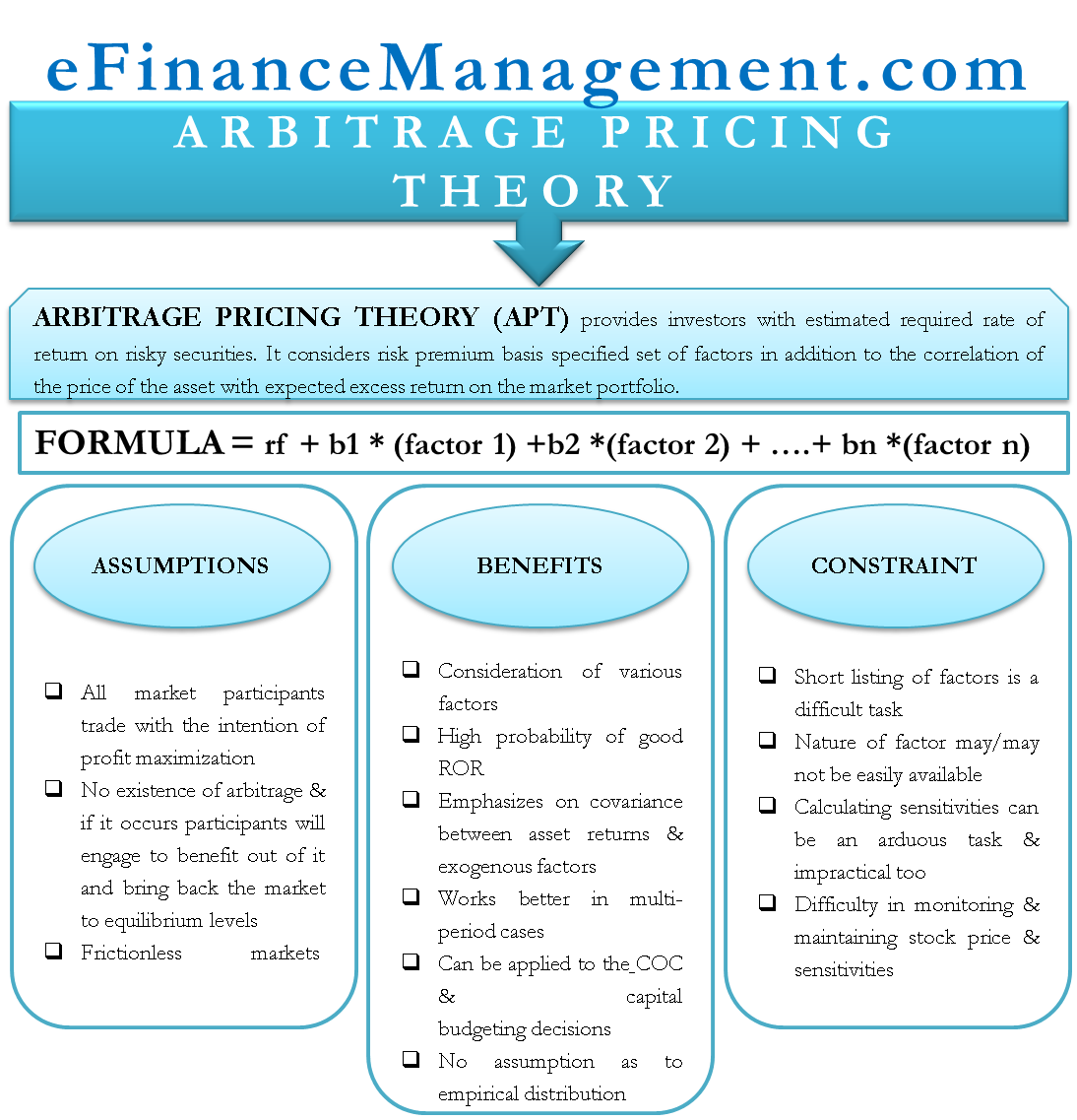
To summarize and visualize the key points from the reading, the three core assumptions of APT are:

1. Factor Model: Asset returns can be described by a linear factor model, where returns are a function of common macroeconomic factors and firm-specific noise.
2. Diversification: Firm-specific (idiosyncratic) risk can be eliminated by holding a well-diversified portfolio.
3. No Arbitrage: No riskless profit opportunities exist among well-diversified portfolios.

These elements are captured in the following infographic.

The APT Pricing Equation

The assumptions we've just discussed lead to a specific mathematical relationship for an asset's expected return. Where CAPM uses a single risk premium (the market risk premium), APT asserts that each systematic risk factor has its own associated risk premium.

The return generating process for an asset i in a K-factor model is:

where:

• $E(r_i)$ is the expected return for asset i.
• $b_{i,j}$ is the sensitivity (factor beta) of asset i's return to factor j.
• ${\tilde{f}}_j$ is the surprise component of the systematic factor j (i.e., the actual factor value minus its expected value). Only the unexpected portion of a factor influences returns, as the expected portion is already priced in.
• $e_i$ is the idiosyncratic or firm-specific random error, with $E(e_i)=0$.

The no-arbitrage condition implies that the expected return, $E(r_i)$, must follow the APT pricing equation:

where:

• $r_f$ is the risk-free rate of return (the return when all betas are zero).
• ${\lambda }_j$ is the factor risk premium for factor j. It represents the extra expected return an investor receives for taking on one unit of risk exposure to that factor.

This equation is the core of APT for practical application. It states that the expected return of an asset is the risk-free rate plus a sum of risk premiums, with each premium determined by the asset's sensitivity to a specific factor.

To see this equation in its formal context, please review the next part of the Duke University PDF.

Conclusion

In this lesson, we have moved beyond the single-factor world of CAPM to explore the more general framework of the Arbitrage Pricing Theory. You now understand that APT is not an equilibrium model but is built on the powerful and intuitive principle of no-arbitrage.

Key Takeaways:

• Multi-Factor Model: APT proposes that an asset's returns are driven by multiple independent systematic risk factors, not just the single market factor of CAPM.
• No-Arbitrage Principle: The theory's foundation is the law of one price. It assumes that arbitrageurs will eliminate any risk-free profit opportunities, forcing assets with the same risk exposures to have the same expected return.
• Weaker Assumptions: APT's assumptions (a factor model for returns, diversifiable idiosyncratic risk, and no arbitrage) are less restrictive than those required for CAPM.
• APT Pricing Equation: The expected return on an asset is the risk-free rate plus the sum of its factor sensitivities ($b_{i,j}$) multiplied by the corresponding factor risk premiums (${\lambda }_j$).

You have now built the conceptual foundation of APT. In our next lesson, we will put this theory into practice by using the APT pricing equation to solve numerical problems and calculate the expected return of an asset given a set of factors and their associated risk measures.