Calculating Expected Returns with Multifactor APT

The APT Pricing Equation in Practice

Let's start by recalling the core APT pricing equation from our last lesson. The expected return for an asset i, denoted $E(R_i)$, is given by:

Where:

• $R_f$ is the risk-free rate of return.
• ${\beta }_{ik}$ is the factor beta, representing the sensitivity of asset i to factor k.
• ${\lambda }_k$ is the risk premium for factor k—the extra return investors demand for bearing the risk associated with that factor.

This formula provides a straightforward method to calculate the expected return of a stock if it is fairly priced according to the model. Let's work through a typical exam-style problem.

Worked Example 1: Calculating Expected Return

Consider the first part of the problem shown in the image below. We are given the risk-free rate, the factor betas for a stock, and the risk premium associated with each factor.

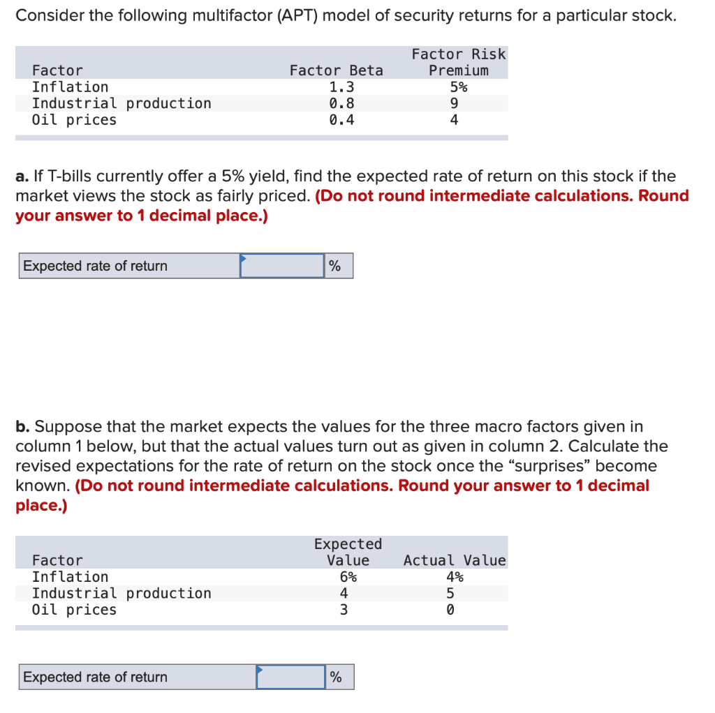
Problem Statement (Part a):
A multifactor APT model for a stock includes three factors: Inflation, Industrial Production, and Oil Prices.

• The factor betas are 1.3, 0.8, and 0.4, respectively.
• The factor risk premiums are 5%, 9%, and 4%, respectively.
• The current risk-free rate (from T-bills) is 5%.

Find the expected rate of return on this stock.

Solution:
We apply the APT pricing equation directly. The expected return is the risk-free rate plus the sum of each factor beta multiplied by its corresponding risk premium.

1. Risk-free Rate: $R_f=5\%$ or $0.05$
2. Inflation Risk Component: ${\beta }_{\text{inflation}}\times {\lambda }_{\text{inflation}}=1.3\times 5\%=6.5\%$ or $0.065$
3. Industrial Production Risk Component: ${\beta }_{\text{prod}}\times {\lambda }_{\text{prod}}=0.8\times 9\%=7.2\%$ or $0.072$
4. Oil Prices Risk Component: ${\beta }_{\text{oil}}\times {\lambda }_{\text{oil}}=0.4\times 4\%=1.6\%$ or $0.016$

Now, we sum these components:

So, if the stock is fairly priced, its expected rate of return is 20.3%.

For a concise walkthrough of a similar calculation, please review the example in the following reading.

From Expected Returns to Actual Returns: The Role of Surprises

The APT pricing equation gives us the expected return, which is the return anticipated by the market based on expected economic conditions. However, the actual return an asset generates will also depend on how economic factors unfold compared to these expectations.

The difference between a factor's actual value and its expected value is called a factor surprise. The full return-generating model in APT separates the expected return from the impact of these surprises:

Where:

• $R_i$ is the actual (or revised) return.
• $E(R_i)$ is the initial expected return we calculated in the previous section.
• $(F_k-E(F_k))$ is the surprise for factor k.
• $e_i$ is the firm-specific (idiosyncratic) return, which we assume to be zero for a well-diversified portfolio.

The following video explains this crucial concept of factor surprises.

Worked Example 2: Calculating a Revised Return

Now that you understand the concept of surprises, let's see how to calculate a revised or actual return in a full numerical example. The next segment of the video provides a clear, step-by-step demonstration.

Let's break down the logic from the video:

1. Calculate Initial Expected Return: This step is identical to our first worked example. You use the formula $E(R)=R_f+\sum {\beta }_k{\lambda }_k$. In the video's example, this came out to 7.1%.
2. Calculate the Surprise Adjustment for Each Factor: For each factor, you calculate ${\beta }_k\times ({\text{Actual Value}}_k-{\text{Expected Value}}_k)$.
3. Calculate the Revised Return: You sum the surprise adjustments and add them to the initial expected return to get the final, revised return.

This two-stage process is a common pattern in APT problems.

Practice Problem

It's time to apply what you've learned. The following reading presents a practice question that mirrors the structure of the "surprise" adjustment calculation we just reviewed.

Conclusion

In this lesson, you have successfully put the Arbitrage Pricing Theory into practice. You have moved beyond the theoretical formula and used it to solve concrete numerical problems, which is a key objective for your CM2 exam preparation.

Key Takeaways:

• Calculating Expected Return: When given a risk-free rate, factor betas, and factor risk premiums, you can calculate the expected return using the equation: $E(R)=R_f+\sum {\beta }_k{\lambda }_k$.
• Calculating Revised Return with Surprises: The actual return generated by an asset depends on how economic factors deviate from expectations. The revised return is calculated by adjusting the initial expected return for these surprises: $R_{\text{revised}}=E(R_{\text{initial}})+\sum {\beta }_k(F_{\text{Actual},k}-F_{\text{Expected},k})$.

You are now proficient in the core calculations related to APT. In our next and final lesson for this module, we will consolidate your knowledge by comparing and contrasting CAPM and APT, evaluating their underlying assumptions, strengths, and weaknesses in practical application.