Introduction
Welcome to the final lesson in our module on Asset Pricing Models. In our last session, we delved into the mechanics of the Arbitrage Pricing Theory (APT), learning how to calculate expected and revised returns using its multifactor framework. You've now mastered the core computations for both the Capital Asset Pricing Model (CAPM) and APT.
Today, we will synthesize this knowledge by directly comparing and contrasting these two foundational models. The goal is to understand not just how they work, but why you might choose one over the other. We will evaluate their underlying assumptions, explore their differences in practical application, and clarify their respective strengths and weaknesses. This comparative analysis is a common topic in finance exams and is essential for developing a nuanced understanding of asset pricing.
The Models at a Glance: Single vs. Multiple Factors
At the most fundamental level, the difference between CAPM and APT lies in how they explain the sources of systematic risk.
Capital Asset Pricing Model (CAPM):
As we've seen, CAPM is a single-factor model. It posits that the only systematic risk that commands a premium is the risk of the overall market. The model's formula is:
Here, the entire systematic risk of asset i is captured by a single sensitivity measure, , relative to the market portfolio.
Arbitrage Pricing Theory (APT):
APT, developed by Stephen Ross, is a multifactor model. It argues that an asset's return is sensitive to various macroeconomic factors, not just the market. The model is expressed as:
APT allows for multiple betas, each capturing the asset's sensitivity to a different systematic risk factor (like inflation, industrial production, or interest rates), with each factor having its own risk premium ().
The following video provides a concise introduction to this core distinction, framing CAPM as a special, single-factor case of the more general APT.
What Is the Arbitrage Pricing Theory?
This short clip from the Investment Management Lab clearly explains the transition from CAPM's single-beta world to APT's multi-beta framework.
Watch from the beginning to this point. Note how APT generalizes the idea of a single market exposure to multiple exposures that can impact asset prices.
A Deeper Dive: Comparing Assumptions
The difference in the number of factors stems from fundamentally different sets of assumptions. As a statistician, you'll find the contrast in their theoretical underpinnings particularly interesting.
To explore this, let's turn to a research paper that directly compares the two models.
[PDF] Model Comparison between CAPM and APT
This paper provides a structured academic comparison of the assumptions and practical limitations of both CAPM and APT.
Please read the following two sections: Start with the section titled "Commonalities and Discrepancies in Assumptions of the CAPM and APT". Read this part carefully to understand both the shared foundations and the key theoretical divergences. Then, read the next section, "Assumption Limitation in Application", which discusses how these theoretical differences translate into practical constraints. Focus on the segment from this paragraph.
Let's summarize the key points from your reading:
Shared Assumptions:
- Asset returns can be described by a linear factor model.
- Investors are rational and risk-averse.
- Unsystematic (idiosyncratic) risk can be eliminated through diversification.
Key Differences in Assumptions:
-
Systematic Risk:
- CAPM: Assumes all systematic risk is captured by a single factor—the market portfolio's excess return.
- APT: Allows for multiple systematic risk factors. It doesn't specify what these factors are, but they are typically macroeconomic variables.
-
The Market Portfolio:
- CAPM: Relies on a theoretical, unobservable "market portfolio" that includes every single asset in the economy. This is a major practical and theoretical weakness, famously pointed out in Roll's Critique.
- APT: Does not require a market portfolio. Its factors are chosen based on their perceived influence on asset prices, making it empirically more testable.
-
Distribution of Asset Returns:
- CAPM: As a mean-variance model, it implicitly assumes either that asset returns are normally distributed or that investors have a quadratic utility function. We know from empirical data that asset returns often exhibit skewness and kurtosis (fat tails), which the normal distribution fails to capture.
- APT: Makes no assumptions about the distribution of asset returns. This makes it theoretically more robust, as it can accommodate the non-normal distributions we observe in reality.
The following video segment reinforces this crucial point about return distributions.
The Arbitrage Pricing Theory and Multifactor Models of Risk and Return (FRM P1 2025– Bk 1 – Chptr 6)
The presenter in this AnalystPrep video highlights the restrictive assumptions of CAPM and how APT relaxes them, particularly concerning the distribution of returns.
Watch the segment from this section. Pay close attention to the discussion about CAPM assuming a normal distribution (or quadratic utility) versus APT making no such assumption.
Practical Application: Simplicity vs. Power
The differences in assumptions lead to significant trade-offs in practice.
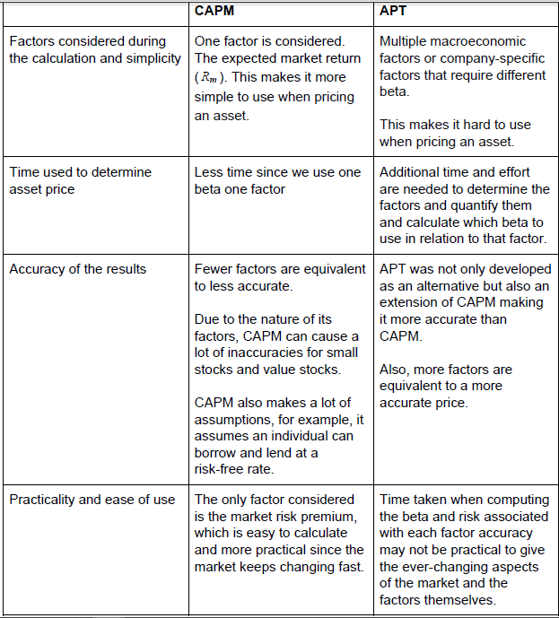
| Feature | Capital Asset Pricing Model (CAPM) | Arbitrage Pricing Theory (APT) |
|---|---|---|
| Ease of Use | Simple. Requires estimating only one beta. The inputs (market return, risk-free rate) are readily available. | Complex. Requires identifying relevant factors, estimating multiple betas, and calculating factor risk premiums. This is a major analytical task. |
| Explanatory Power | Lower. Its single factor may fail to explain returns for assets sensitive to other systematic risks. | Higher. By incorporating multiple factors, it can provide a more nuanced and accurate explanation of asset returns. |
| Flexibility | Rigid. The model is fixed with the market factor. | Flexible. The user can choose the factors believed to be most relevant for the asset or portfolio being analyzed. |
| Hedging | Limited. Only allows for managing overall market exposure by adjusting beta. | Powerful. Allows for hedging specific systematic risks (e.g., inflation risk) by creating portfolios with zero beta for that factor. |
This summary table highlights the central trade-off: CAPM offers simplicity at the cost of realism, while APT offers realism and power at the cost of complexity.
The Power of Hedging with APT
One of the most significant practical advantages of APT is its application in risk management. Because it breaks down systematic risk into multiple components, it allows an investor to selectively hedge against specific risks. For example, a pension fund concerned about rising inflation could use APT to construct a portfolio that is neutral to inflation shocks while remaining exposed to other growth-oriented factors. This level of granular risk control is impossible with CAPM.
The following clip explains this powerful application.
The Arbitrage Pricing Theory and Multifactor Models of Risk and Return (FRM P1 2025– Bk 1 – Chptr 6)
This part of the video explains how the multifactor structure of APT can be used to hedge against specific systematic risks, a key practical advantage over CAPM.
Watch from this segment. The core idea is that you can take an offsetting (short) position in a factor portfolio to neutralize your exposure to that specific risk.
From Abstract Theory to a Practical Model: Fama-French
A common criticism of APT is that the theory itself doesn't specify which factors to use. In response, researchers have developed specific, empirically-driven multifactor models. The most famous of these is the Fama-French Three-Factor Model, which extends CAPM by adding two factors:
- Size (SMB - Small Minus Big): The tendency for smaller companies to outperform larger ones.
- Value (HML - High Minus Low): The tendency for companies with high book-to-market ratios (value stocks) to outperform those with low ratios (growth stocks).
The Fama-French model is a direct, practical application of APT's principles and is widely used in both academia and the investment industry, demonstrating the evolution from CAPM's single-factor world.
Conclusion
In this lesson, we have systematically compared CAPM and APT, completing our study of the major asset pricing models. You should now be able to articulate the trade-offs between them clearly.
Key Takeaways:
- Structure: CAPM is a simple, single-factor model based on market risk. APT is a flexible, multifactor model that can incorporate various macroeconomic risks.
- Assumptions: APT is built on fewer and less restrictive assumptions than CAPM, notably avoiding the need for a theoretical market portfolio and assumptions about the normality of returns.
- Practicality: CAPM is easier to implement but may be less accurate. APT is more complex and data-intensive to apply but offers greater explanatory power and sophisticated risk management capabilities like factor-specific hedging.
- Relationship: Many practitioners view CAPM as a simplified, special case of the more general APT framework.
With this, we conclude the module on Asset Pricing Models. You have progressed from understanding individual risk measures to portfolio theory, and finally to the models that tie an asset's risk to its expected return.
In our next module, we will shift gears from these static equilibrium models to the dynamic modeling of asset prices over time. Leveraging your background in probability theory, we will begin exploring the world of stochastic processes, starting with the geometric Brownian motion model that forms the bedrock of modern option pricing.