Modeling Asset Prices with Geometric Brownian Motion (GBM)

From Deterministic Growth to Random Walks

Before we introduce randomness, let's start with a simple, deterministic model of growth. Imagine an asset, like money in a savings account, that grows at a continuously compounded rate.

The quantpie video channel offers an excellent derivation of the differential equation for this process, starting from first principles.

As the video explains, if a quantity $S_t$ (our asset price) grows at a constant rate $\mu$, its evolution can be described by the ODE:

This can also be written in differential form as $d{S}_t=\mu S_{t}dt$. This equation states that the change in the asset price over an infinitesimally small time interval $dt$ is proportional to its current price $S_t$. This is our model's deterministic drift component.

However, we know that real asset prices don't follow such a smooth, predictable path. They are subject to random shocks. To model this, we need to introduce a stochastic element.

Introducing the Random Component: Brownian Motion

The standard tool for modeling continuous-time randomness in finance is the Wiener process, also known as Brownian motion. Given your background, you are likely familiar with its core properties, but let's briefly recap them in the context of finance:

• Starting Point: It starts at zero: $W_0=0$.
• Continuous Paths: The path of $W_t$ is continuous; it doesn't have any jumps.
• Independent Increments: The change over any time interval, $W_{t+u}-W_t$, is independent of the process's history before time $t$.
• Normal Increments: The increments are normally distributed with a mean of 0 and a variance equal to the time elapsed: $W_{t+u}-W_t\sim N(0,u)$.

While Brownian motion captures randomness, it's not a suitable model for stock prices on its own. For instance, a standard Wiener process can take on negative values, but stock prices cannot be negative due to limited liability. Furthermore, we expect the magnitude of random price swings to be proportional to the stock's price level (e.g., a $1 change is more significant for a $10 stock than for a $1000 stock).

This is where Geometric Brownian Motion comes in.

The Stochastic Differential Equation for GBM

Geometric Brownian Motion combines the deterministic drift from our first model with a random component based on a Wiener process, where both components are proportional to the current asset price. This structure elegantly resolves the issues mentioned above.

The dynamic of an asset price $S_t$ following a GBM is described by the following Stochastic Differential Equation (SDE):

Let's break this down:

• $d{S}_t$: The infinitesimal change in the stock price at time $t$.
• $\mu S_{t}dt$: This is the drift term. It's the deterministic part of the price change.
  • $\mu$ is the instantaneous expected return or drift rate of the asset price.
  • This term implies that, on average, the price is expected to grow by a percentage $\mu$ over time.
• $\sigma S_{t}d{W}_t$: This is the diffusion term or stochastic part.
  • $\sigma$ is the instantaneous volatility, which measures the magnitude of the random fluctuations.
  • $d{W}_t$ is the increment of a Wiener process, representing the source of randomness. Because $W_t$ has increments with variance $dt$, you can think of $d{W}_t$ as being a random draw from a normal distribution with mean 0 and variance $dt$.

The Quant Next channel provides a concise summary of this SDE within the broader context of stochastic calculus.

Interpreting the GBM Model

The name "Geometric" Brownian Motion comes from the fact that the drift and volatility are proportional to the current state of the process, $S_t$. We can make this even clearer by rearranging the SDE:

This form shows that the model is not for the absolute price change, but for the percentage price change, $d{S}_t/S_t$. It states that the instantaneous percentage return is composed of a constant expected return ($\mu dt$) and a random shock with constant volatility ($\sigma d{W}_t$). This ensures that as the stock price grows, the magnitude of its fluctuations also grows, which is a realistic feature. It also guarantees that the stock price will remain positive (if it starts positive).

The following document from Ohio State University provides a formal definition of GBM and its SDE, reinforcing what we've just discussed.

The image below illustrates what sample paths generated by a GBM process look like. It shows two paths with different drift ($\mu$) and volatility ($\sigma$) parameters.

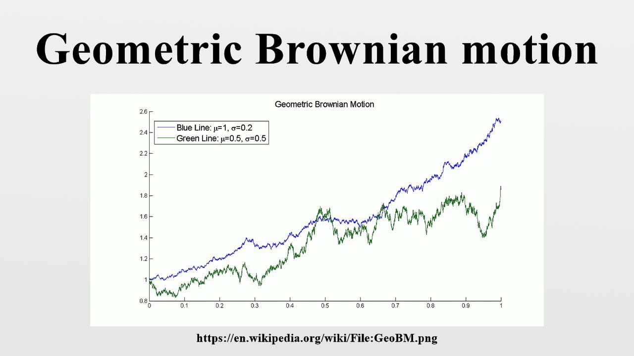
Notice how the blue line, with its higher drift-to-volatility ratio, exhibits a more pronounced upward trend. The green line is much more volatile and its trend is less apparent. This visual helps build intuition for how the parameters $\mu$ and $\sigma$ govern the behavior of the asset price path.

Conclusion

In this lesson, we have taken a significant step from static models to the dynamic world of continuous-time finance. We established the Stochastic Differential Equation for Geometric Brownian Motion, the workhorse model for asset prices.

Key Takeaways:

• Asset price dynamics can be modeled by combining a deterministic trend (drift) with a random component (diffusion).
• The SDE for Geometric Brownian Motion is $d{S}_t=\mu S_{t}dt+\sigma S_{t}d{W}_t$.
• The parameter $\mu$ is the instantaneous expected return, dictating the trend.
• The parameter $\sigma$ is the instantaneous volatility, dictating the magnitude of random fluctuations.
• The model assumes that percentage returns, not absolute returns, are random, which keeps prices positive and makes the size of price moves proportional to the price level.

The SDE tells us how the price changes over an infinitesimal time step. But how do we use it to find the price $S_T$ at some future time $T$? To do that, we need to "solve" this SDE. Standard calculus rules don't apply due to the stochastic term $d{W}_t$. This requires a new tool: Itô's Lemma, the fundamental theorem of stochastic calculus. In our next lesson, we will learn how to apply Itô's Lemma to solve the GBM equation and find the distribution of future stock prices.