Deriving and Interpreting the Security Market Line (SML)

Introduction

Welcome back! In our last lesson, we established the foundational assumptions of the Capital Asset Pricing Model (CAPM). We concluded that in the idealized world defined by those assumptions, all investors hold the same "market portfolio" of risky assets, and therefore, the only risk that commands a reward is systematic risk—the risk that cannot be diversified away. This risk, as we know, is measured by beta ( $β$ ).

This lesson brings that theoretical conclusion to life by introducing the Security Market Line (SML). The SML is the graphical and mathematical embodiment of the CAPM. It answers the crucial question: "For a given amount of systematic risk, what return should an investor expect?" We will explore the elegant logic behind the SML's famous formula, break down its components, and learn how to use it as a powerful benchmark to evaluate whether an individual asset is fairly priced, underpriced, or overpriced.

The Logic of the Security Market Line

The derivation of the SML hinges on a core principle of equilibrium: in a perfectly competitive market, the reward-to-risk ratio should be the same for all assets. If one asset offered a better reward for its risk than another, rational investors would flock to it, bidding up its price and driving down its future return until the ratios were equal again.

The CAPM formalizes this idea. The "reward" for any investment is its expected return in excess of the risk-free rate. The "risk" is the investment's contribution to the total risk of the market portfolio.

For the market portfolio (M) itself:
- The reward is the market risk premium: $E (r_{M}) - r_{f}$ .
- The risk is the variance of the market: $σ_{M}^{2}$ .
- The market's reward-to-risk ratio is: $\frac{E ( r _{M} ) - r _{f}}{σ _{M}^{2}}$ .
For any individual asset (i):
- The reward is its risk premium: $E (r_{i}) - r_{f}$ .
- Its contribution to the market's risk is not its own variance, but its covariance with the market: $Cov (r_{i}, r_{M})$ . Given your background in statistics, you'll recognize that this covariance term captures how asset i moves with the market, which is precisely its systematic risk contribution.

In equilibrium, the two reward-to-risk ratios must be equal:

\frac{E ( r _{i} ) - r _{f}}{Cov ( r _{i} , r _{M} )} = \frac{E ( r _{M} ) - r _{f}}{σ _{M}^{2}}

Now, we just need to rearrange this equation to solve for the expected return of asset i, $E (r_{i})$ :

E (r_{i}) - r_{f} = \frac{Cov ( r _{i} , r _{M} )}{σ _{M}^{2}} \times [E (r_{M}) - r_{f}]

You will immediately recognize the fraction $\frac{Cov ( r _{i} , r _{M} )}{σ _{M}^{2}}$ as the definition of beta ( $β_{i}$ ). Substituting $β_{i}$ gives us the celebrated SML equation:

E (r_{i}) = r_{f} + β_{i} [E (r_{M}) - r_{f}]

This elegant equation states that the expected return on any asset is the sum of the risk-free rate plus a risk premium, which is the asset's systematic risk ( $β_{i}$ ) multiplied by the market price of risk ( $E (r_{M}) - r_{f}$ ).

For a more detailed look at this derivation, you can refer to the following resource.

[PDF] Portfolio Theory And Equilibrium In Capital Markets - Actex

This study manual provides the mathematical steps that formalize the logic we just discussed.

Focus your reading on two key parts. First, review the section titled Expected returns on individual securities. This walks through the reward-to-risk ratio logic to arrive at the SML equation. Then, read the short section that follows, The security market line, which defines the SML and distinguishes it from the CML.

Visualizing the SML: The Graph and Its Components

The SML equation is a simple linear relationship, which makes it perfect for graphical representation. The Wall Street Prep article below offers a very clear explanation of the SML graph and its formula.

Security Market Line (SML) | Formula + Slope of Graph

This article provides an excellent, practical breakdown of the SML, its formula, and its graphical interpretation.

Please read the first five sections, from the introduction down to the end of the "Slope" section. Pay close attention to the definitions of the axes, the y-intercept, and the slope.

Let's break down the key features of the SML graph, as shown below.

This graph plots the Security Market Line, showing the linear relationship between an asset's systematic risk (Beta) and its Expected Return as predicted by the CAPM.

X-Axis: Systematic Risk ( $β$ ): This axis measures how much an asset's return tends to move with the overall market. A beta of 1 means the asset moves in line with the market. A beta of 1.5 means it's 50% more volatile than the market. A beta of 0.5 means it's 50% less volatile.
Y-Axis: Expected Return ( $E (r)$ ): This is the required rate of return for an asset with a given beta.
Y-Intercept: Risk-Free Rate ( $r_{f}$ ): The line starts at the risk-free rate. This is logical: an asset with a beta of 0 has no systematic risk, so an investor should expect to earn no more and no less than the risk-free return.
Slope: Market Risk Premium ( $E (r_{M}) - r_{f}$ ): The slope of the SML represents the "price of risk." It tells you how much additional expected return the market demands for each additional unit of systematic risk you take on.

A key point to remember is the distinction between the SML and the Capital Market Line (CML) from our previous module. The CML plots expected return against total risk (standard deviation, $σ$ ) and applies only to efficient portfolios. The SML plots expected return against systematic risk ( $β$ ) and applies to any individual asset or portfolio, whether efficient or not.

This video offers a great visual explanation of the SML and its components using a practical example.

Explaining the Capital Asset Pricing Model (CAPM) & Security Market Line (SML)

This video from Ryan O'Connell provides a clear, step-by-step walkthrough of the CAPM formula and the SML graph.

First, watch from the beginning to the overview of the CAPM formula to see how the SML equation is built from its four variables. Then, jump to the section on the SML graph from the start of the SML explanation to see how the line is plotted and how specific assets (like the market and Microsoft) find their place on it.

Interpreting the SML: Finding Undervalued and Overvalued Assets

The true power of the SML is as a benchmark. The line itself represents the return that an asset should offer, according to the CAPM, given its risk. By comparing an asset's actual expected return (which you might estimate from your own research) to the required return on the SML, we can determine if it's a good investment.

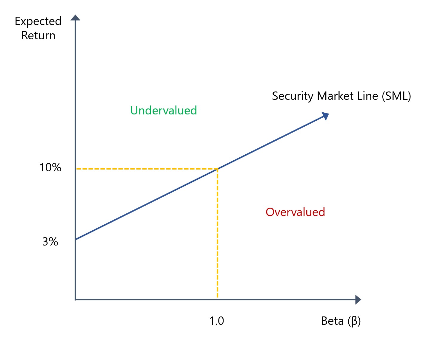
This graph illustrates how the position of an asset relative to the SML indicates whether it is undervalued or overvalued.

Assets on the SML: An asset whose expected return plots directly on the SML is considered fairly priced. Its expected return is exactly what it should be for the amount of systematic risk it carries. In perfect equilibrium, all assets would lie on this line.
Assets above the SML: An asset whose expected return plots above the SML is considered undervalued. It offers a higher return than is required for its level of risk. This is a potential "buy" signal. The vertical distance from the asset's plotted point to the SML is called its alpha ( $α$ ), a measure of its excess return.
Assets below the SML: An asset whose expected return plots below the SML is considered overvalued. It offers a lower return than is required for its level of risk. This is a potential "sell" or "avoid" signal. Such an asset would have a negative alpha.

The following video provides an excellent summary of this interpretation.

Capital Market Line (CML) vs Security Market Line (SML)

This clip from Dr. Ronald Moy's channel clearly explains how to interpret assets that fall above or below the SML.

Watch the segment from the explanation of over- and undervaluation. He provides a concise definition for each case, relating it back to the risk-return trade-off.

Conclusion

In this lesson, we bridged the gap from the abstract assumptions of the CAPM to its most important practical application: the Security Market Line. We have seen that the SML is more than just a line on a graph; it is a powerful statement about the nature of risk and return in financial markets.

Key Takeaways:

The SML is the graphical representation of the CAPM, derived from the equilibrium condition that all assets must offer the same reward-to-risk ratio.
The SML equation is $E (r_{i}) = r_{f} + β_{i} [E (r_{M}) - r_{f}]$ .
It plots Expected Return ( $E (r)$ ) against Systematic Risk ( $β$ ).
The line's y-intercept is the risk-free rate ( $r_{f}$ ), and its slope is the market risk premium ( $E (r_{M}) - r_{f}$ ).
The SML serves as a benchmark for asset valuation:
- Assets plotting above the SML are considered undervalued (positive alpha).
- Assets plotting below the SML are considered overvalued (negative alpha).
- Assets plotting on the SML are considered fairly priced (zero alpha).

Now that we understand the SML's logic and interpretation, we are ready to put it to work. In our next lesson, we will focus on applying the SML formula to solve practical problems, such as calculating the expected return for a stock and quantifying its performance using Jensen's alpha. This will align directly with the numerical, application-focused approach you prefer for your exam preparation.

Recommended resources

Introduction

The Logic of the Security Market Line

Visualizing the SML: The Graph and Its Components

Interpreting the SML: Finding Undervalued and Overvalued Assets

Conclusion