Minimum Variance Portfolio: Matrix Approach

1. The N-Asset Case in Matrix Notation

To handle a portfolio of N assets efficiently, we must first express its characteristics using vectors and matrices. Let's define the key components:

• Expected Returns Vector ($\mathbf{\mu }$): An $N\times 1$ column vector where the $i$-th element is the expected return of asset $i$, ${\mu }_i$. $$\mathbf{\mu }=\left(\begin{array}{c}{\mu }_1\\ {\mu }_2\\ ⋮\\ {\mu }_N\end{array}\right)$$
• Portfolio Weights Vector ($\mathbf{w}$): An $N\times 1$ column vector where the $i$-th element, $w_i$, is the proportion of wealth invested in asset $i$. $$\mathbf{w}=\left(\begin{array}{c}{w}_1\\ w_2\\ ⋮\\ w_N\end{array}\right)$$
• Covariance Matrix ($\mathbf{\Sigma }$): An $N\times N$ matrix where the element in the $i$-th row and $j$-th column is the covariance between asset $i$ and asset $j$, ${\sigma }_{ij}$. The diagonal elements, ${\sigma }_{ii}$, are the variances, ${\sigma }_i^2$. $$\mathbf{\Sigma }=\left(\begin{array}{cccc}{\sigma }_1^2& {\sigma }_{12}& \cdots & {\sigma }_{1N}\\ {\sigma }_{21}& {\sigma }_2^2& \cdots & {\sigma }_{2N}\\ ⋮& ⋮& \ddots & ⋮\\ {\sigma }_{N1}& {\sigma }_{N2}& \cdots & {\sigma }_N^2\end{array}\right)$$

With this notation, the portfolio's expected return ${\mu }_p$ and variance ${\sigma }_p^2$ become elegantly simple expressions:

• Portfolio Expected Return: ${\mu }_p={\sum }_{i=1}^N{w}_i{\mu }_i={\mathbf{w}}^T\mathbf{\mu }$
• Portfolio Variance: ${\sigma }_p^2={\sum }_{i=1}^N{\sum }_{j=1}^N{w}_i{w}_j{\sigma }_{ij}={\mathbf{w}}^T\mathbf{\Sigma }\mathbf{w}$

The following reading formalizes this setup. As a statistician, you will recognize the variance formula as a quadratic form, which is central to multivariate statistical analysis.

Our goal is to find the Global Minimum Variance Portfolio. This means we must find the weight vector $\mathbf{w}$ that minimizes the portfolio variance ${\sigma }_p^2$. However, there is one crucial constraint: the weights must sum to 1, ensuring we are fully invested. In matrix notation, this constraint is written as ${\mathbf{w}}^{T}1=1$, where $1$ is an $N\times 1$ vector of ones.

So, the problem is formally stated as:
Minimize ${\sigma }_p^2={\mathbf{w}}^T\mathbf{\Sigma }\mathbf{w}$
Subject to ${\mathbf{w}}^{T}1=1$

2. Solving the Optimization Problem

This is a classic constrained optimization problem, which can be solved using the method of Lagrange multipliers. The goal is to find the minimum of a function subject to a constraint. We'll construct a new function, the Lagrangian $L$, and find its unconstrained minimum, which will correspond to the constrained minimum of our original function.

The Lagrangian function for our problem is:

Here, $\lambda$ is the Lagrange multiplier. To find the minimum, we take the partial derivatives of $L$ with respect to each weight $w_i$ (which is equivalent to differentiating with respect to the vector $\mathbf{w}$) and with respect to $\lambda$, and set them to zero. This gives us a system of $N+1$ linear equations.

The following resource walks through this derivation, showing how it leads to a system of equations that can be solved in a single step using matrix inversion.

As shown in the reading, the first-order conditions lead to the following block matrix system:

Solving this system for the vector $\left(\begin{array}{c}\mathbf{w}\\ \lambda \end{array}\right)$ gives us the optimal weight vector $\mathbf{w}$ for the GMVP.

3. The Explicit Formula and a Practical Example

While the block matrix approach works, algebraic manipulation of the first-order conditions yields a more direct and elegant formula for the GMVP weights:

Let's break this down:

• The numerator, ${\mathbf{\Sigma }}^{-1}1$, calculates a vector of weights that are not yet scaled. ${\mathbf{\Sigma }}^{-1}$ is the inverse of the covariance matrix, often called the precision matrix in statistics.
• The denominator, $1^T({\mathbf{\Sigma }}^{-1}1)$, is a scalar value (a single number). It is the sum of all the elements in the unscaled weight vector from the numerator.
• Dividing the vector by this scalar ensures that the final weights in ${\mathbf{w}}_{\text{GMVP}}$ sum to 1, thus satisfying our constraint.

This formula is the analytical solution to the problem that numerical tools like Excel's Solver tackle through iteration. The following video demonstrates how such a solver is used in practice. While it doesn't use our matrix formula directly, it perfectly illustrates the problem we are solving: minimizing risk subject to the full investment constraint.

Let's see what a final solution looks like for a 5-asset portfolio.

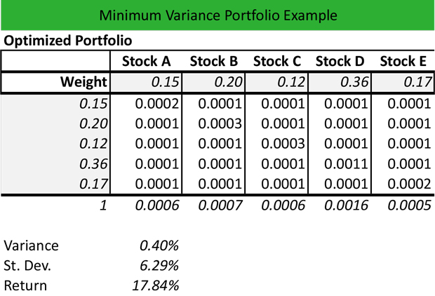
In this example, the optimal weights (0.15, 0.20, 0.12, 0.36, 0.17) were found by applying the formula we just discussed to the given covariance matrix. This resulted in a portfolio with a minimum possible variance of 0.40% (or a standard deviation of 6.29%).

Conclusion

Today, we have made a significant leap from a visual, two-asset framework to a powerful, analytical N-asset solution. You now have the mathematical tool to solve for the portfolio with the lowest possible risk from any number of assets, provided you have their covariance matrix.

The key takeaways from this lesson are:

• The GMVP problem is formulated as a constrained optimization: minimize ${\mathbf{w}}^T\mathbf{\Sigma }\mathbf{w}$ subject to ${\mathbf{w}}^{T}1=1$.
• This problem can be solved analytically using the method of Lagrange multipliers.
• The solution for the GMVP weights has a compact and elegant form in matrix notation: ${\mathbf{w}}_{\text{GMVP}}=\frac{{\mathbf{\Sigma }}^{-1}1}{1^T{\mathbf{\Sigma }}^{-1}1}$. This provides a direct, non-iterative method for finding the optimal weights.

We have now analytically located the "tip" of the Markowitz bullet. In our next lesson, we will expand this method to find any other optimal portfolio on the efficient frontier. We will do this by introducing a second constraint: a specific target for the portfolio's expected return. This will equip us to trace out the entire efficient frontier mathematically.