In our previous lesson, we established the fundamental formulas for calculating the expected return and variance of a single portfolio composed of two risky assets. You learned that while portfolio return is a simple weighted average, portfolio risk is more complex, with the correlation between assets playing a pivotal role in diversification.
Today, we will take that foundation and build upon it significantly. Instead of looking at just one combination of weights, we will explore the entire universe of possible portfolios that can be created from two assets. By calculating the risk and return for every possible weighting scheme, we will be able to plot the complete set of investment opportunities. This will lead us to one of the most important concepts in modern finance: the efficient frontier. By the end of this lesson, you will be able to plot this frontier and, more importantly, interpret what it tells us about making optimal investment choices.
1. From a Single Point to a Universe of Portfolios
In the last lesson, we took a set of asset characteristics (means, variances, correlation) and a single pair of weights () to calculate a single risk-return point (). Now, imagine we systematically vary the weights. For example, we could start with 100% in Asset B (), then move to 1% in A and 99% in B, then 2% in A and 98% in B, and so on, all the way to 100% in Asset A. We can even consider short-selling, where one weight is negative and the other is greater than 1.
For each of these infinite combinations of weights, we can calculate a corresponding () pair. If we plot all of these points on a graph with risk () on the x-axis and return () on the y-axis, we trace out a curve. This curve represents the complete set of all feasible portfolios and is often called the investment possibilities set or the portfolio frontier.
The following resource provides an excellent, numerically-driven walkthrough of this exact process. It starts with the characteristics of two assets and then generates a table of different portfolio weights and their resulting risk-return coordinates, culminating in a plot of the portfolio frontier.
11.2 Portfolios of Two Risky Assets
This chapter from "Introduction to Computational Finance and Financial Econometrics with R" demonstrates how to generate and visualize the set of all possible portfolios from two risky assets.
Please read the section The set of feasible portfolios. As you read, focus on the table that shows different values for the weights x_A and x_B and the corresponding values for portfolio mean \mu_p and standard deviation \sigma_p. Then, carefully examine the resulting plot, often called the "Markowitz bullet," which visualizes these risk-return trade-offs.
As you saw, the plot of all possible portfolios forms a distinct curve that is "pulled" or "bowed" to the left. This curvature is the graphical representation of the diversification benefit we discussed previously.
2. A Practical Demonstration: Plotting the Frontier
Seeing the concept in a textbook is one thing; building it yourself provides a different level of understanding. The next video demonstrates how to perform these calculations and generate the efficient frontier plot using a common tool, Microsoft Excel. This hands-on approach directly aligns with your goal of practical application.
The video starts with raw asset price data to calculate the necessary inputs (mean, standard deviation, covariance), then proceeds to calculate the risk and return for various portfolio weightings, and finally plots them.
Graph The Efficient Frontier And Capital Allocation Line In Excel
This video, "Graph The Efficient Frontier And Capital Allocation Line In Excel" from the channel of Ryan O'Connell, CFA, FRM, provides a practical step-by-step guide.
Please watch the following two segments: First, watch from 02:18 to 05:05. This part demonstrates how to create a table of different portfolio weights and then apply the formulas for portfolio return and standard deviation to calculate the risk-return coordinates for each portfolio. Notice how the formulas you learned in the previous lesson are applied repeatedly for each weight combination. Next, watch from 05:49 to 06:30. Here, the presenter takes the calculated data and uses a scatter plot to visually create the portfolio frontier.
3. The Influence of Correlation
The "bowing" of the portfolio frontier to the left is a direct consequence of the correlation between the assets being less than perfect (). The degree of this curvature is determined entirely by the correlation coefficient. Let's examine the limiting cases and what lies between them.
The following video masterfully illustrates how the shape of the investment possibilities set changes for different levels of correlation.
CFA® Level I Portfolio Management - Minimum Variance Portfolios and Efficient Frontier
This video from PrepNuggets, "CFA® Level I Portfolio Management - Minimum Variance Portfolios and Efficient Frontier", clearly visualizes the impact of correlation.
Watch the segment from 01:18 to 05:30. It will guide you through three key scenarios: Perfect Positive Correlation (\rho = +1): You'll see that the portfolio frontier is a straight line. There is no curvature and thus no risk reduction from diversification. The portfolio's risk is simply the weighted average of the individual asset risks. Perfect Negative Correlation (\rho = -1): This is the ideal (though unrealistic) scenario for diversification. The frontier bows so far to the left that it touches the y-axis, meaning it's possible to form a portfolio with zero risk. Zero Correlation (\rho = 0): This is a more practical example showing significant curvature and demonstrating that even with uncorrelated (not necessarily negatively correlated) assets, diversification provides substantial risk reduction.
The key insight here, which is fundamental to portfolio theory, is that as long as two assets are not perfectly positively correlated, combining them in a portfolio can reduce risk below the level of a simple weighted average. The lower the correlation, the greater the diversification benefit and the more pronounced the curvature of the portfolio frontier.
4. Isolating the "Efficient" Portfolios
We have now plotted the full set of all feasible portfolios. But are all of them desirable? Consider the plot below.
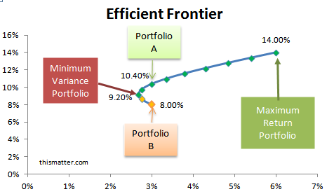
Imagine you are at the risk level corresponding to Portfolio B. You could achieve a much higher expected return for the exact same amount of risk by moving vertically up to Portfolio A. Stated differently, for any portfolio on the lower half of the curve (like Portfolio B), there is another portfolio on the upper half that is strictly better because it either offers a higher return for the same risk or the same return for less risk.
Therefore, a rational, risk-averse investor would only ever consider portfolios that lie on the upper boundary of the feasible set. This upper part of the curve is what we call the Efficient Frontier.
The turning point of the curve, labeled "Minimum Variance Portfolio," is the portfolio with the absolute lowest risk possible when combining these two assets. It is often called the Global Minimum Variance Portfolio (GMVP). The efficient frontier consists of the GMVP and all portfolios above it on the curve.
The following segment provides a formal definition and interpretation of the efficient frontier.
CFA® Level I Portfolio Management - Minimum Variance Portfolios and Efficient Frontier
Let's return to the PrepNuggets video to formalize these concepts.
Please watch from 05:30 to 07:36. This section distinguishes between the minimum variance frontier (the whole curve) and the efficient frontier (the top half). It clearly explains the logic of why a risk-averse investor would only choose portfolios on the efficient frontier and formally defines the Global Minimum Variance Portfolio.
Conclusion
In this lesson, we moved from analyzing a single portfolio to mapping the entire universe of possibilities for two assets. This allowed us to visualize the trade-offs between risk and return and to identify the set of optimal portfolios.
Here are the main takeaways:
- By varying the weights of two assets and calculating the resulting portfolio risk and return, we can plot the investment possibilities set, or portfolio frontier.
- The shape of this frontier is determined by the correlation between the assets. A lower correlation leads to more curvature, representing a greater diversification benefit.
- The efficient frontier is the upper portion of the portfolio frontier, starting from the Global Minimum Variance Portfolio (GMVP).
- For any given level of risk, the efficient frontier provides the portfolio with the maximum possible expected return. Consequently, these are the only portfolios a rational, risk-averse investor would consider.
In today's lesson, we identified the efficient frontier visually for a simple two-asset case. In our next lesson, we will begin to generalize this powerful concept. We will introduce the use of matrix algebra to mathematically solve for a key point on this curve—the Global Minimum Variance Portfolio—for a portfolio containing N risky assets, setting the stage for more complex portfolio optimization problems.