Portfolio Expected Return and Variance

Welcome to the first lesson of our new module on Mean-Variance Portfolio Theory. In our previous module, we concluded by establishing a formal basis for why diversification is beneficial, using the concept of coherent risk measures. We saw that the sub-additivity of Expected Shortfall mathematically captures the idea that the risk of a combined portfolio should be no greater than the sum of its parts.

Today, we will begin to put that principle into practice. We will move from the abstract concept of diversification to the concrete mechanics of building a portfolio. You will learn how to quantify the two most important characteristics of any investment portfolio: its expected return and its risk, measured by variance. Your background in statistics will be a great asset here, as we will be applying familiar concepts like expected value, variance, and covariance to the financial context of asset returns.

By the end of this lesson, you will be able to calculate the expected return and variance for a portfolio composed of two risky assets, laying the essential groundwork for constructing optimal portfolios.

1. The Ingredients of a Portfolio

The theory we are about to explore, developed by Harry Markowitz in the 1950s, is a cornerstone of modern finance. It provides a mathematical framework for assembling a portfolio of assets to maximize expected return for a given level of risk. The first step is to master the formulas for a simple two-asset portfolio.

A portfolio's characteristics are determined by three things:

The individual properties of each asset (their expected returns and variances).
The way the assets move in relation to each other (their covariance or correlation).
The proportion of our capital allocated to each asset (the portfolio weights).

Portfolio Expected Return

Let's consider a portfolio with two assets, Asset A and Asset B. We'll denote their expected returns as $E [R_{A}]$ and $E [R_{B}]$ , respectively. Let $w_{A}$ and $w_{B}$ be the weights, or proportions, of our total funds invested in each asset, such that $w_{A} + w_{B} = 1$ .

The expected return of the portfolio, $E [R_{p}]$ , is simply the weighted average of the expected returns of the individual assets. From your probability theory background, you'll recognize this as calculating the expected value of a linear combination of random variables.

E [R_{p}] = w_{A} E [R_{A}] + w_{B} E [R_{B}]

This relationship is linear and straightforward. If you increase the weight of the asset with the higher expected return, the portfolio's expected return increases proportionally.

Portfolio Risk (Variance)

Calculating the portfolio's risk is more interesting. The risk, measured by variance ( $σ_{p}^{2}$ ), is not a simple weighted average of the individual asset variances. The interaction between the assets, captured by their covariance, plays a crucial role.

The formula for the variance of a two-asset portfolio is:

σ_{p}^{2} = w_{A}^{2} σ_{A}^{2} + w_{B}^{2} σ_{B}^{2} + 2 w_{A} w_{B} Cov (R_{A}, R_{B})

Where $σ_{A}^{2}$ and $σ_{B}^{2}$ are the variances of Asset A and Asset B, and $Cov (R_{A}, R_{B})$ is the covariance of their returns. This formula is the standard result for the variance of a weighted sum of two correlated random variables.

Since covariance can be difficult to interpret, we often express it in terms of the correlation coefficient, $ρ_{A B}$ . Recall the relationship: $Cov (R_{A}, R_{B}) = ρ_{A B} σ_{A} σ_{B}$ , where $σ_{A}$ and $σ_{B}$ are the standard deviations. Substituting this into the variance formula gives us a more intuitive version:

σ_{p}^{2} = w_{A}^{2} σ_{A}^{2} + w_{B}^{2} σ_{B}^{2} + 2 w_{A} w_{B} ρ_{A B} σ_{A} σ_{B}

This equation is the mathematical heart of diversification. The final term, the "interaction term," shows how the portfolio's total risk is affected by how the two assets move together.

2. A Guided Walkthrough

The following video provides a clear, step-by-step explanation of these formulas and works through a numerical example for each. This will help solidify your understanding of how to apply them.

Diversification with Two Assets

This video, "Diversification with Two Assets" by Eric Kelley, provides a concise walkthrough of calculating portfolio return and variance.

Please watch the following segments: First, from 03:05 to 05:02, which covers the portfolio return calculation with an example. Then, from 05:02 to 09:02, which details the formula for portfolio variance and emphasizes the critical role of correlation. Finally, watch the worked example for portfolio variance from 09:02 to 11:20.

3. The Power of Correlation: A Deeper Dive

As the video highlighted, the correlation coefficient, $ρ_{A B}$ , is the key to understanding diversification. Let's explore its impact with a detailed example.

Scenario:
Suppose we are building a portfolio with two stocks, Stock X and Stock Y.

Stock X: Expected Return $E [R_{X}] = 8%$ , Standard Deviation $σ_{X} = 12%$
Stock Y: Expected Return $E [R_{Y}] = 15%$ , Standard Deviation $σ_{Y} = 20%$
Weights: We invest 70% in Stock X ( $w_{X} = 0.7$ ) and 30% in Stock Y ( $w_{Y} = 0.3$ ).
Correlation: The correlation between the returns of X and Y is $ρ_{X Y} = 0.2$ .

Step 1: Calculate the Portfolio's Expected Return

Using the weighted average formula:

E [R_{p}] = w_{X} E [R_{X}] + w_{Y} E [R_{Y}] = (0.7 \times 0.08) + (0.3 \times 0.15)

E [R_{p}] = 0.056 + 0.045 = 0.101 = 10.1%

Step 2: Calculate the Portfolio's Variance and Standard Deviation

Now, we apply the full variance formula:

σ_{p}^{2} = w_{X}^{2} σ_{X}^{2} + w_{Y}^{2} σ_{Y}^{2} + 2 w_{X} w_{Y} ρ_{X Y} σ_{X} σ_{Y}

Plugging in the numbers:

σ_{p}^{2} = (0.7)^{2} (0.12)^{2} + (0.3)^{2} (0.20)^{2} + 2 (0.7) (0.3) (0.2) (0.12) (0.20)

σ_{p}^{2} = (0.49) (0.0144) + (0.09) (0.04) + (0.084) (0.024)

σ_{p}^{2} = 0.007056 + 0.0036 + 0.002016 = 0.012672

The portfolio's standard deviation is the square root of the variance:

σ_{p} = 0.012672 \approx 0.1126 = 11.26%

Notice that the portfolio's risk ( $11.26%$ ) is less than the risk of Stock X ( $12%$ ) and significantly less than the risk of Stock Y ( $20%$ ). It is even less than the weighted average of the individual standard deviations ( $0.7 \times 12% + 0.3 \times 20% = 14.4%$ ). This reduction in risk is the diversification benefit in action.

What happens if correlation changes?

Let's see how the portfolio risk changes if the correlation were different, keeping everything else the same.

If $ρ_{X Y} = 1$ (Perfect Positive Correlation): The assets move in perfect lock-step.
$σ_{p}^{2} = 0.007056 + 0.0036 + 2 (0.7) (0.3) (1) (0.12) (0.20) = 0.020736$ $σ_{p} = 0.020736 = 0.144 = 14.4%$
In this specific case, the portfolio risk is exactly the weighted average of the individual risks. There is no diversification benefit.
If $ρ_{X Y} = - 1$ (Perfect Negative Correlation): The assets move in perfect opposition.
$σ_{p}^{2} = 0.007056 + 0.0036 + 2 (0.7) (0.3) (- 1) (0.12) (0.20) = 0.000624$ $σ_{p} = 0.000624 \approx 0.025 = 2.5%$
Here, the diversification benefit is immense. The offsetting movements of the two assets cancel out most of the risk.

This demonstrates that the lower the correlation, the greater the potential for risk reduction.

This relationship is visualized in the chart below. Each curve represents the possible risk-return combinations for a two-asset portfolio, given a different correlation coefficient.

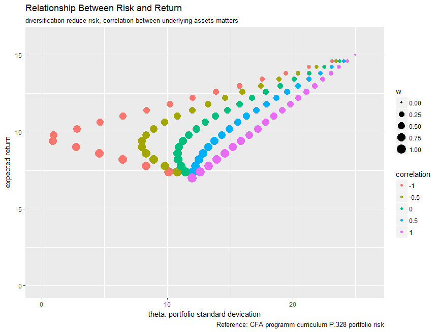
This plot shows the expected return (y-axis) versus the portfolio standard deviation (x-axis) for various combinations of two assets. Each colored curve corresponds to a different correlation coefficient between the assets. Notice how lower correlations (e.g., -1, -0.5) bend the curve further to the left, offering portfolios with much lower risk for a given return.

As you can see, when the correlation is +1 (pink dots), the risk-return trade-off is a straight line. As the correlation decreases, the curve bows out to the left, indicating that it's possible to achieve the same return with lower risk. This "bowing" is the visual representation of diversification.

For further reference and more worked examples, the following resource from AnalystPrep is excellent. It's geared towards actuarial exams and presents the material clearly.

Mean-Variance Portfolio Theory for CFA/FRM Exams

This guide from AnalystPrep provides clear definitions and several exam-style numerical examples.

Please review the following sections: Expected Return of a Portfolio, which includes a concise example. Risk of a Portfolio, which presents the variance formula and a detailed example. Example 3, which works through another complete calculation of both portfolio return and risk.

Conclusion

In this lesson, we have established the fundamental mathematical tools for analyzing a two-asset portfolio. You learned how to combine the individual characteristics of assets to determine the overall characteristics of your portfolio.

Here are the key takeaways:

The expected return of a portfolio is the weighted average of the expected returns of its constituent assets.
The variance (risk) of a portfolio depends not only on the individual asset variances but crucially on the covariance or correlation between them.
The formula $σ_{p}^{2} = w_{A}^{2} σ_{A}^{2} + w_{B}^{2} σ_{B}^{2} + 2 w_{A} w_{B} ρ_{A B} σ_{A} σ_{B}$ is the engine of diversification.
Lower correlation between assets leads to greater risk reduction, illustrating the core principle of not putting all your eggs in one basket.

In our next lesson, we will build directly on today's calculations. We will take these risk and return values for every possible weighting scheme and plot them to create the efficient frontier, a concept that will allow us to visually identify the set of all optimal portfolios.