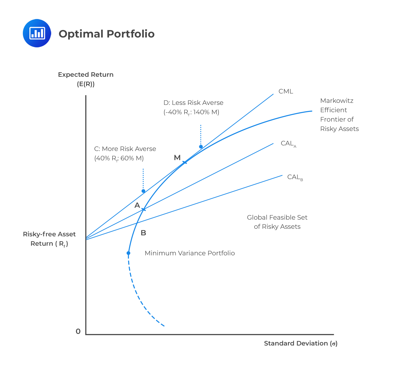
In our last lesson, we took a significant step by developing an analytical method to find the Global Minimum Variance Portfolio (GMVP) for any number of assets. We formulated it as an optimization problem with a single constraint—that all portfolio weights must sum to one—and solved it using Lagrange multipliers. This gave us the precise location of one special point: the very tip of the "Markowitz bullet."
Today, we will generalize that approach to find any optimal portfolio along the entire efficient frontier. To do this, we will introduce a second constraint: a specific target for the portfolio's expected return. By solving this new, doubly-constrained optimization problem, you will be able to trace out the full set of efficient portfolios, equipping you with the complete mathematical framework for Markowitz portfolio selection among risky assets.
1. Formulating the Efficient Frontier Problem
Recall that the efficient frontier represents the set of portfolios that offer the highest possible expected return for a given level of risk (variance). In the previous lesson, we framed this as minimizing risk. We will continue with that approach, but now we add a condition that the portfolio must achieve a pre-determined expected return.
The problem, therefore, has the same objective function but two constraints:
- The portfolio weights must sum to 1 (the "fully invested" constraint).
- The portfolio's expected return must equal a specific target level, which we'll call .
Using the matrix notation from our last session, the problem is formally stated as:
Minimize:
Subject to:
Here, is the vector of portfolio weights we are solving for, is the covariance matrix, is the vector of expected asset returns, and is a vector of ones.
2. Solving with Two Lagrange Multipliers
Because we now have two constraints, our Lagrangian function will require two multipliers. Let's call them and . The method remains the same: we combine the objective function and the constraints into a single equation and find its stationary point.
The Lagrangian is:
The intuition here is a direct extension of the single-multiplier case. At the optimal point, the gradient of the objective function (variance) must be a linear combination of the gradients of the two constraint functions. The Lagrange multipliers, and , are the coefficients of this linear combination.
For a powerful visual refresher on this core concept, the following video explains the geometric idea of parallel gradients that underpins the Lagrangian method.
Constrained Optimization: Intuition behind the Lagrangian
This video from MATLAB provides a fantastic and intuitive explanation of how Lagrange multipliers work for constrained optimization.
I recommend watching from the geometric intuition. The key idea is that at an optimal point, the contour of the objective function is tangent to the constraint line. This means their gradient vectors must be parallel, which is precisely what the Lagrangian equation captures.
The following video from MIT OpenCourseWare walks through the setup of this exact problem, showing how to formulate the Lagrangian and derive the first-order conditions to find the solution.
This lecture clip from "Finance Theory I" at MIT lucidly presents the core Markowitz optimization problem.
Please watch from the derivation. Focus on these key steps: How the problem is set up to minimize volatility subject to a mean return target. The construction of the Lagrangian with two multipliers for the two constraints. The concept that solving this for different target returns (\alpha_0 in the video) traces out the efficient frontier, which takes the shape of a parabola.
3. The Matrix Solution and the Efficient Frontier
As the video explained, taking the partial derivatives of the Lagrangian with respect to , , and and setting them to zero gives us a system of linear equations. This system can be neatly expressed in a block matrix format, which is a straightforward extension of the GMVP solution from our last lesson.
The following reading provides the detailed derivation and the final matrix equation.
Chapter 1 Portfolio Theory with Matrix Algebra
This document from the University of Washington provides a rigorous yet clear step-by-step derivation for finding efficient portfolios using matrix algebra.
Please read the section titled "Finding efficient portfolios". Pay close attention to how the two constraints lead to a larger (N+2) \times (N+2) block matrix system: \begin{pmatrix} 2\boldsymbol{\Sigma} & \boldsymbol{\mu} & \mathbf{1} \\ \boldsymbol{\mu}^T & 0 & 0 \\ \mathbf{1}^T & 0 & 0 \end{pmatrix} \begin{pmatrix} \mathbf{w} \\ \lambda_1 \\ \lambda_2 \end{pmatrix} = \begin{pmatrix} \mathbf{0} \\ \mu_p^* \\ 1 \end{pmatrix} Notice the structure: the top-left corner is similar to the GMVP problem, but we've added rows and columns corresponding to the new expected return constraint. Solving this system for \mathbf{w} gives you the weights for the efficient portfolio that has an expected return of \mu_p^*.
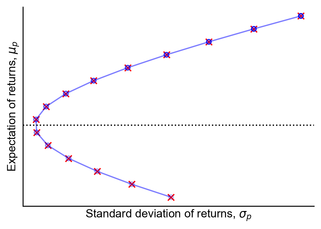
By solving this matrix equation for various target returns (specifically, for any greater than or equal to the GMVP's expected return), we can calculate the weights for every portfolio on the efficient frontier. Plotting the resulting expected returns () against their corresponding standard deviations () generates the classic "Markowitz bullet."
4. A Note on Practical Constraints
The elegant matrix solution we've derived assumes we can take any weights, positive or negative (i.e., short selling is allowed). In practice, many portfolio managers face additional constraints, such as:
- Long-only constraints: All weights must be non-negative ().
- Holding constraints: Limits on the maximum weight for any single asset.
- Turnover constraints: Limits on how much the portfolio can be changed from one period to the next.
When these inequality constraints are introduced, we can no longer use simple matrix inversion. The problem becomes a more general quadratic programming problem, which requires numerical algorithms (like Excel's Solver) to find the solution. However, the fundamental setup—minimizing variance subject to constraints—remains the same. The MIT video briefly discusses this.
The same MIT video provides a brief overview of practical constraints used in real-world portfolio optimization.
For context, you can optionally watch the segment from portfolio constraints. This highlights how our theoretical model can be extended to accommodate real-world complexities.
Conclusion
In this lesson, you have learned how to generalize the search for the optimal portfolio beyond just the GMVP. By adding a second constraint for a target expected return, you can now mathematically define and solve for any portfolio on the efficient frontier.
The key takeaways are:
- Finding an efficient portfolio is an optimization problem: minimize variance subject to a target return and the full investment constraint.
- This problem is solved using the method of Lagrange multipliers, now requiring two multipliers for the two constraints.
- The solution can be found by solving a single, expanded block matrix equation.
- By iterating through different target return values (), we can trace out the entire efficient frontier of risky assets.
We have now fully characterized the investment opportunity set for risky assets. Our next step is to see what happens when we introduce a risk-free asset. As you will see, this dramatically simplifies the investment decision and leads to a powerful new concept: the Capital Market Line.