Estimating Lognormal Model Parameters from Historical Prices

Introduction

In our previous lesson, we successfully solved the stochastic differential equation for Geometric Brownian Motion (GBM), arriving at the explicit formula for a future stock price, $S_{T}$ . This revealed the foundational principle that stock prices are assumed to follow a lognormal distribution. The solution, which should be fresh in your mind, is:

S_{T} = S_{0} exp ((μ - \frac{1}{2} σ^{2}) T + σ W_{T})

This formula is a powerful theoretical tool, but its practical use hinges entirely on the values of the drift parameter $μ$ and the volatility parameter $σ$ . Today, we bridge the gap between this theory and real-world application. Our objective is to learn how to estimate these crucial parameters from historical stock price data. As a statistician, you'll recognize this as a classic parameter estimation problem: we have a model and a dataset, and we need to find the model parameters that best fit the data.

The Foundation: Log-Returns

The key to estimating $μ$ and $σ$ lies in the properties of logarithmic returns, which we established in the last lesson. We found that the continuously compounded return over a period $T$ , $ln (S_{T} / S_{0})$ , is normally distributed. Let's adapt this insight for discrete time steps, which is how we receive real-world data (e.g., daily closing prices).

Let's consider a series of historical stock prices $S_{0}, S_{1}, S_{2}, \dots, S_{n}$ recorded at regular intervals of length $Δ t$ . For daily data, $Δ t$ would represent one day. We define the log-return for each period as:

u_{i} = ln (\frac{S _{i}}{S _{i - 1}}) = ln (S_{i}) - ln (S_{i - 1})

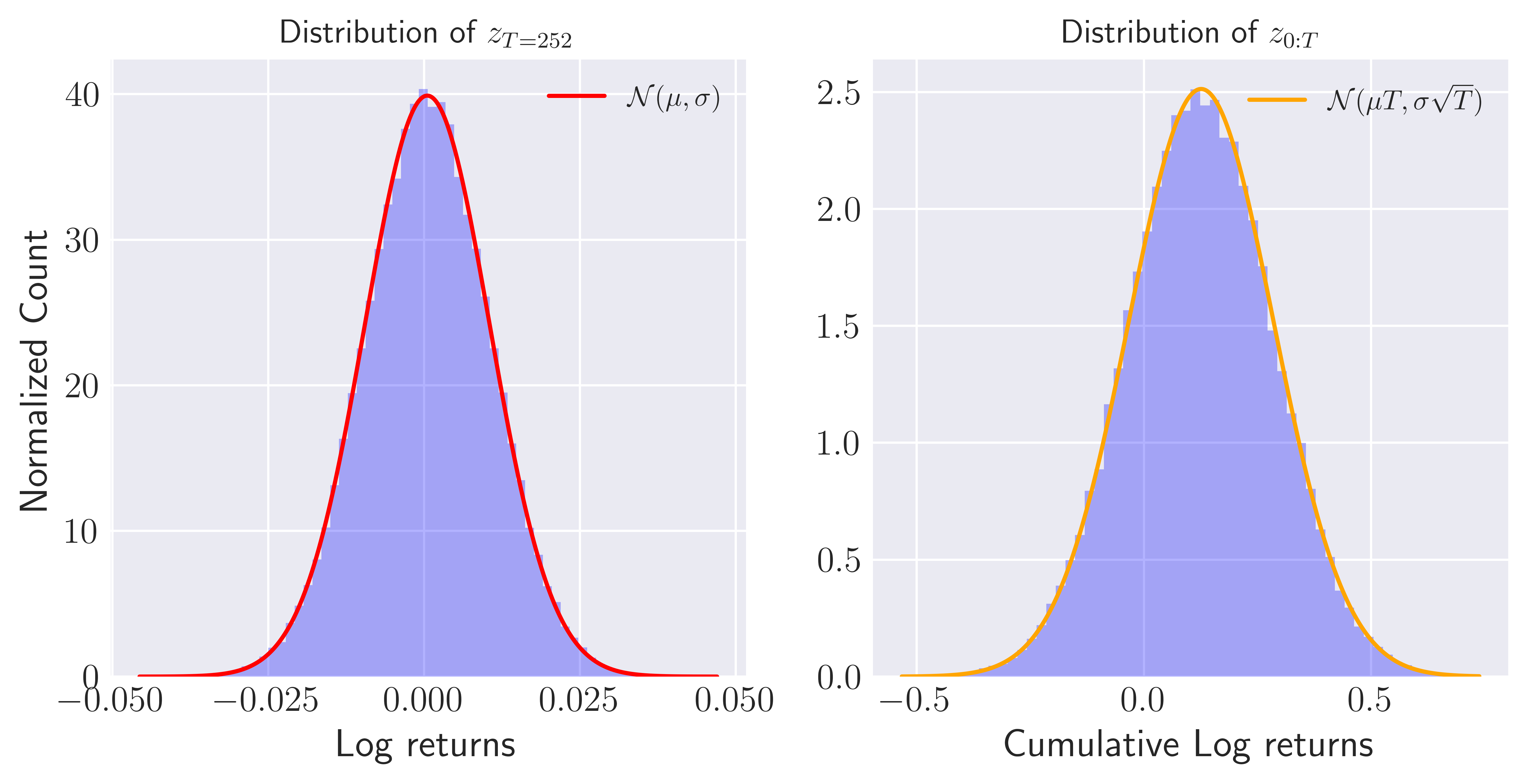
From the solution to the GBM SDE, we can say that over a small time step $Δ t$ , each log-return is an independent draw from a normal distribution:

u_{i} \sim N ((μ - \frac{1}{2} σ^{2}) Δ t, σ^{2} Δ t)

This is the central pillar of our estimation strategy. We have transformed the complex, non-stationary price series $S_{t}$ into a series of log-returns $u_{i}$ that are assumed to be independent and identically distributed (i.i.d.) normal random variables. Your expertise in probability theory makes the next step straightforward: we can use standard statistical methods to estimate the mean and variance of this normal distribution.

Estimating Daily Parameters

Let's denote the mean and variance of the daily log-returns as $m^$ and $s^^{2}$ , respectively. These are simply the sample mean and sample variance of our calculated log-return series $u_{1}, u_{2}, \dots, u_{n}$ :

Sample Mean: $m^= \frac{1}{n} \sum_{i = 1}^{n} u_{i}$
Sample Variance: $s^^{2} = \frac{1}{n - 1} \sum_{i = 1}^{n} (u_{i} - m^)^{2}$

These sample statistics are our estimators for the parameters of the daily log-return distribution.

$m^$ is our estimate for $(μ - \frac{1}{2} σ^{2}) Δ t$ .
$s^^{2}$ is our estimate for $σ^{2} Δ t$ .

The following video provides a detailed mathematical derivation that shows why the sample mean and sample variance of log-returns are the correct estimators for the parameters of the underlying GBM model.

Brownian Motion Share Price Modelling

This video, "Brownian Motion Share Price Modelling" from Mathematics with Plymouth University, rigorously walks through the mathematics linking the GBM model to the distribution of log-returns.

Please watch the section from this derivation. The presenter takes the logarithm of the GBM price formula and analyzes the difference between consecutive log-prices. The key conclusion, reached around this point, is that the expected value of these log-differences is the drift parameter (in his notation) and the variance is the volatility parameter squared. This justifies using the sample mean and sample variance as estimators. Note that the video assumes a time step of 1, so the parameters derived are per-period (e.g., daily) parameters, which we will annualize next.

Annualizing the Parameters

While we estimate parameters from daily data, the conventions in finance require $μ$ and $σ$ to be expressed as annualized figures. To do this, we need to scale our daily estimates. Let's assume there are $T_{A}$ trading days in a year (a common value is $T_{A} = 252$ ). This means our time step in years is $Δ t = 1/ T_{A}$ .

1. Estimating Volatility ( $σ$ )

We start with our estimate for the variance of daily log-returns:

σ^_{daily}^{2} = s^^{2}

Since variance scales linearly with time, the annualized variance is:

σ^^{2} = σ^_{daily}^{2} \times T_{A} = s^^{2} \times T_{A}

Therefore, the annualized volatility is:

σ^= s^^{2} \times T_{A} = s^\times T_{A}

This "square-root-of-time" rule for scaling volatility is one of the most fundamental concepts in quantitative finance.

2. Estimating Drift ( $μ$ )

The process for the drift is slightly more involved. We first estimate the daily mean of the log-returns:

Mean_{daily} = m^

This $m^$ is our estimate for the term $(μ - \frac{1}{2} σ^{2}) Δ t$ . Let's call this term $ν Δ t$ .

ν Δ t^= m^⟹ ν^= \frac{m ^}{Δ t} = m^\times T_{A}

Now we use the relationship $μ = ν + \frac{1}{2} σ^{2}$ and substitute our annualized estimates:

μ^= ν^+ \frac{1}{2} σ^^{2} = (m^\times T_{A}) + \frac{1}{2} (s^^{2} \times T_{A})

This gives us the annualized drift parameter consistent with the SDE $d S_{t} = μ S_{t} d t + σ S_{t} d W_{t}$ .

A Practical Walkthrough

Let's solidify this with a practical example, showing how you would perform these calculations in a tool like Excel.

Step 1: Obtain Historical Prices
First, you gather a time series of adjusted closing prices for an asset.

Step 2: Calculate Daily Log-Returns
In a new column, calculate the daily log-return for each day (except the first). The formula for cell D5 in the image below would be LN(C5/C4).

Step 3: Calculate Sample Statistics
Calculate the sample mean ( $m^$ ) and sample standard deviation ( $s^$ ) of the entire column of log-returns.

AVERAGE(D5:Dn) would give $m^$ .
STDEV.S(D5:Dn) would give $s^$ . The .S is important as it specifies a sample standard deviation, using $n - 1$ in the denominator, which is what we need.

This spreadsheet demonstrates the calculation of daily log returns from closing prices. The highlighted formula shows the use of `STDEV.S` to calculate the sample standard deviation of these log returns, which is our $\hat{s}$.

Step 4: Annualize the Parameters
Using the calculated $m^$ and $s^$ , and assuming $T_{A} = 252$ :

Annualized Volatility: $σ^= s^\times 252$
Annualized Drift: $μ^= (m^\times 252) + 0.5 \times σ^^{2}$ (where $σ^^{2} = s^^{2} \times 252$ )

The following video provides a clear, step-by-step guide to performing these calculations in Excel.

Stock Annual Return & Standard Deviation in Excel | FREE FILE

The video "Stock Annual Return & Standard Deviation in Excel" by Ryan O'Connell, CFA, FRM is a perfect practical guide for this process.

First, watch how to calculate daily logarithmic returns. This corresponds to our Step 2. Next, observe the calculation of the annual standard deviation (\hat{\sigma}). The presenter correctly calculates the sample standard deviation of daily returns and scales it by the square root of 252. This is exactly our formula for \hat{\sigma}. Finally, review the calculation of the annual return. The method shown here, SUM(daily returns) * 252 / N, is equivalent to AVERAGE(daily returns) * 252, which is the first part of our drift calculation (\hat{m} \times T_A). Note that for a complete GBM drift estimate, you would still need to add the \frac{1}{2}\hat{\sigma}^2 term. The video calculates the average log-return, which corresponds to \hat{\nu}, not the full SDE drift \hat{\mu}. This is a common simplification, but for the CM2 exam, it's crucial to know the full formula.

Clarifying Different 'Drift' Notations

It is essential to address a common point of confusion regarding the drift parameter $μ$ . You will encounter different, seemingly contradictory formulas for estimating it. The discrepancy arises from two different (but related) ways of expressing the model.

SDE Form: $d S_{t} = μ S_{t} d t + σ S_{t} d W_{t}$
- Here, $μ$ is the instantaneous expected return. The corresponding log-return mean is $(μ - \frac{1}{2} σ^{2}) Δ t$ .
- To estimate this $μ$ , you must use the formula we derived: $μ^= (m^\times T_{A}) + \frac{1}{2} σ^^{2}$ .
Solution Form: $S_{T} = S_{0} exp (ν T + σ W_{T})$
- Here, $ν = μ - \frac{1}{2} σ^{2}$ is the drift of the log-price process.
- The mean of the log-returns directly estimates $ν Δ t$ . So, $ν^= m^\times T_{A}$ .

Many practitioners work directly with $ν$ because it's simpler to estimate. However, the parameter $μ$ in the standard SDE definition requires the addition of the $\frac{1}{2} σ^{2}$ term. For your exam, you must be clear which parameter is being asked for.

This reading from a quantitative finance forum provides an excellent discussion of exactly this issue, confirming the correct approach.

equities - Simulate stock prices with Geometric Brownian Motion ...

This StackExchange answer directly addresses the confusion between different ways of calculating \mu and \sigma.

Focus on the section of the answer that starts with the solution to the GBM model: log-returns are normal. The author shows that the mean of the log-returns is (\mu - 0.5\sigma^2)\delta t. Then, pay close attention to the formulas for calibrating the model. The author explains how to get \sigma and then \mu from the estimated mean and variance of the log-returns (the formula for mu). This confirms the method we have just discussed and highlights why simply taking the average of returns is insufficient for estimating the \mu of the SDE.

This image visually confirms our core assumption. The histogram on the left shows the distribution of daily log returns from a simulation, which closely matches a normal distribution. The histogram on the right shows that the cumulative log returns over a longer period are also normally distributed, with a larger variance, as predicted by our model ($\sigma^2 T$).

Conclusion

In this lesson, we have built the essential practical skill of calibrating our theoretical GBM model to real-world data. By leveraging the normality of log-returns, a property you are well-equipped to handle, we can use simple sample statistics to find the model's parameters.

Key Takeaways:

The estimation of GBM parameters is based on the assumption that daily logarithmic returns $u_{i} = ln (S_{i} / S_{i - 1})$ are i.i.d. normal random variables.
We first calculate the sample mean ( $m^$ ) and sample standard deviation ( $s^$ ) of the historical daily log-returns.
These daily statistics are then annualized to get the conventional drift ( $μ$ ) and volatility ( $σ$ ) parameters.
- Annualized Volatility: $σ^= s^T_{A}$
- Annualized Drift: $μ^= (m^\times T_{A}) + \frac{1}{2} σ^^{2}$
It is crucial to distinguish between the drift of the SDE ( $μ$ ) and the drift of the log-price process ( $ν = μ - \frac{1}{2} σ^{2}$ ), as their estimation methods differ by the $\frac{1}{2} σ^{2}$ term.

Now that we have a fully specified model, we can use it to make quantitative statements about the future. In our next lesson, we will put our estimated parameters to work, using the lognormal model to calculate probabilities of future stock prices reaching certain levels and to determine price quantiles for risk management.

Recommended resources