Deriving Lognormal Stock Prices from GBM

Solving the Stochastic Differential Equation

The SDE for the log-price is effectively a recipe for how $\ln (S_t)$ changes over an infinitesimal time step $dt$. To find the value at a future time $T$, we need to "sum up" all these small changes from our starting point at time $t=0$. In the continuous-time world, this summation is an integration.

We can express the SDE in its integral form:

Let's solve this term by term:

1. The left-hand side is the integral of a perfect differential, which simply evaluates to the change in the process between the endpoints: $\ln (S_T)-\ln (S_0)$.
2. The first term on the right is an integral of a constant with respect to time, which is straightforward: $\left(\mu -\frac{1}{2}{\sigma }^2\right)T$.
3. The second term is a stochastic integral. For our purposes, we can state that the integral of a constant $\sigma$ with respect to a Wiener process $W_t$ is $\sigma {\int }_0^{T}d{W}_t=\sigma (W_T-W_0)$. By definition, a standard Wiener process starts at zero, so $W_0=0$. The term becomes $\sigma W_T$.

Putting these pieces together, we get the solution for the log-price at time $T$:

Rearranging to isolate $\ln (S_T)$ gives:

Finally, to get the solution for the stock price $S_T$ itself, we just need to exponentiate both sides:

This is the explicit solution to the Geometric Brownian Motion SDE. It gives us a direct formula for the price of an asset at any future time $T$, based on its starting price $S_0$, its parameters $\mu$ and $\sigma$, and the outcome of a single random variable, $W_T$.

The following brief reading provides a clear summary of this derivation.

The Lognormal Property of Stock Prices

Now, let's analyze the solution from a probabilistic perspective. The formula for $\ln (S_T)$ can be rewritten as:

The term on the left, $\ln (S_T/S_0)$, is the continuously compounded return of the stock over the period from 0 to $T$.

The right-hand side is a sum of a constant and a scaled Wiener process. From your background in probability theory, you know that a standard Wiener process at time $T$, $W_T$, is a normally distributed random variable with mean 0 and variance $T$. That is, $W_T\sim N(0,T)$.

Consequently, the entire right-hand side is a linear transformation of a normal random variable, which means it is also normally distributed. Let's find its mean and variance:

• Mean: $\mathbb{E}\left[\left(\mu -\frac{1}{2}{\sigma }^2\right)T+\sigma W_T\right]=\left(\mu -\frac{1}{2}{\sigma }^2\right)T+\sigma \mathbb{E}[W_T]=\left(\mu -\frac{1}{2}{\sigma }^2\right)T$
• Variance: $\text{Var}\left[\left(\mu -\frac{1}{2}{\sigma }^2\right)T+\sigma W_T\right]=\text{Var}(\sigma W_T)={\sigma }^2\text{Var}(W_T)={\sigma }^{2}T$

Therefore, we have the crucial result that the log-return is normally distributed:

By definition, a random variable whose logarithm is normally distributed is said to have a lognormal distribution. Thus, the future stock price $S_T$ is lognormally distributed. This property is foundational to quantitative finance and is the reason GBM is also called the lognormal model.

The following video segment neatly summarizes both the derivation and this probabilistic interpretation.

Interpreting the Solution

The lognormal model has several appealing features for modeling asset prices:

• Positivity: Since the exponential function is always positive, $S_T$ can never be negative, matching the limited liability of stocks.
• Right Skew: The distribution is skewed to the right, reflecting the fact that while downside is limited to zero, the potential for upside is, in theory, unlimited.
• Parameter Roles: The parameters $\mu$ and $\sigma$ have clear roles. The drift $\mu$ governs the overall trend, while the volatility $\sigma$ controls the magnitude of the random fluctuations around that trend.

The image below illustrates this. It shows two simulated paths of GBM.

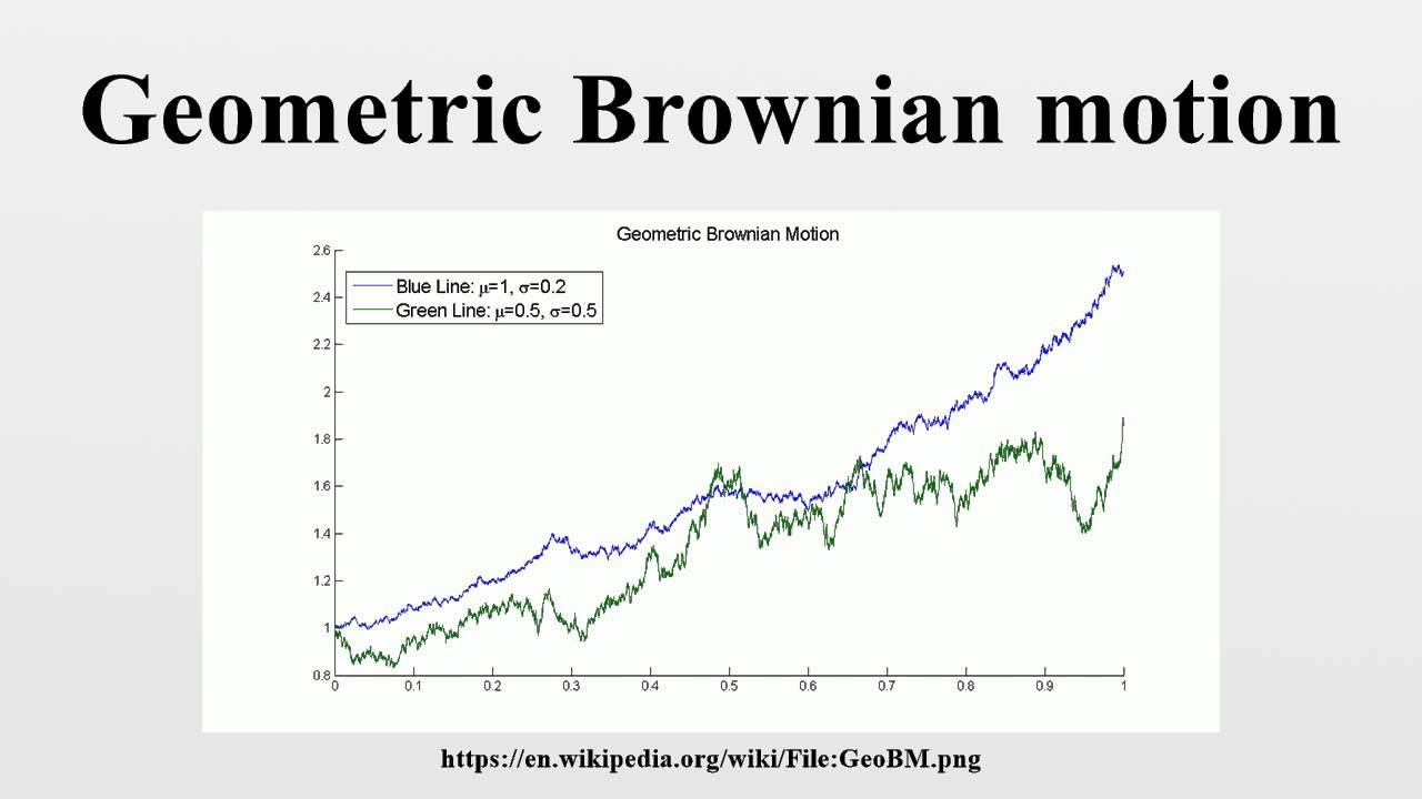
As you can see, the higher drift $\mu$ for the blue line pushes its average path higher than the green line's. Meanwhile, the higher volatility $\sigma$ for the green line causes it to exhibit much wider and more frequent swings.

Simulating Stock Prices

The explicit solution for $S_T$ allows us to simulate future stock price paths, which is essential for pricing complex derivatives and for risk management. To simulate a price at a small time step $\Delta t$ from the current price $S_t$, we use a discretized version of our solution:

Here, $Z$ is a random draw from a standard normal distribution, $N(0,1)$, and the $\sqrt{\Delta t}$ term comes from the fact that the variance of the Wiener increment $W_{t+\Delta t}-W_t$ is $\Delta t$. By generating a sequence of random draws for $Z$, we can build an entire price path step-by-step.

This video clip provides a nice numerical example.

Conclusion

This lesson marks a significant milestone in our journey. By solving the SDE for Geometric Brownian Motion, we have moved from an abstract model of infinitesimal price changes to a concrete, predictive formula for future asset prices.

Key Takeaways:

• The SDE for Geometric Brownian Motion has an explicit analytical solution:
  $S_T=S_0\exp \left(\left(\mu -\frac{1}{2}{\sigma }^2\right)T+\sigma W_T\right)$
• This solution implies that the continuously compounded return, $\ln (S_T/S_0)$, is normally distributed with mean $(\mu -\frac{1}{2}{\sigma }^2)T$ and variance ${\sigma }^{2}T$.
• Consequently, the future stock price $S_T$ follows a lognormal distribution. This is a cornerstone of modern quantitative finance.
• The parameters $\mu$ (drift) and $\sigma$ (volatility) control the trend and randomness of the price paths, respectively.

We now have a powerful theoretical model. But how do we connect it to the real world? In our next lesson, we will address this by learning how to estimate the crucial parameters $\mu$ and $\sigma$ from historical stock price data. This will bridge the gap between theory and practice, enabling us to apply the lognormal model to actual financial assets.