Lognormal Stock Price Model: Probabilities and Quantiles

The Lognormal Property: Our Analytical Engine

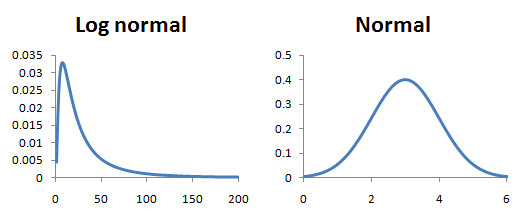
Let's begin by revisiting the cornerstone of our model. We established that if a stock price $S_t$ follows GBM, its future value at time $T$, denoted $S_T$, is lognormally distributed. More specifically, the natural logarithm of the future price is normally distributed. This is the key that unlocks our ability to perform calculations.

The distribution is given by:

Equivalently, we can express this in terms of the continuously compounded return over the period:

Here, $S_0$ is the current price, $T$ is the time horizon in years, and $\mu$ and $\sigma$ are the annualized drift and volatility parameters we learned to estimate in the previous lesson.

This relationship means that while the stock price $S_T$ itself has a skewed, lognormal distribution, its logarithm $\ln (S_T)$ has the familiar, symmetric bell-curve shape of a normal distribution.

Calculating Probabilities of Future Stock Prices

A common question in finance and for your CM2 exam is to find the probability that a stock price will be above or below a certain level at a future date. For example, what is $P(S_T>K)$ for some strike price $K$?

Since we know the distribution of $\ln (S_T)$, the procedure is a standard application of normal distribution theory:

1. Transform the Inequality: Since the natural logarithm is a monotonically increasing function, the inequality $S_T>K$ is equivalent to $\ln (S_T)>\ln (K)$.
2. Standardize: We convert our normally distributed variable $\ln (S_T)$ into a standard normal variable $Z\sim N(0,1)$ using the formula $Z=(X-\text{mean})/\text{std.dev.}$.

Let's define the mean and standard deviation of $\ln (S_T)$:

• Mean: $m=\ln (S_0)+\left(\mu -\frac{1}{2}{\sigma }^2\right)T$
• Variance: $v={\sigma }^{2}T$
• Standard Deviation: $s=\sigma \sqrt{T}$

The probability calculation becomes:

This simplifies to:

The expression on the right is just a number, which we can look up in a standard normal cumulative distribution function (CDF) table, denoted by $\Phi (z)$. Remember that $P(Z>z)=1-P(Z\le z)=1-\Phi (z)$.

The following document provides a clear, step-by-step example of this exact calculation.

Let's work through another example, this time using a typical exam problem format.

Let's break down the solution in the image:

• Parameters: $\mu =0.16$, $\sigma =0.40$, $T=10$. The dividend yield $\delta$ is 0 for a non-dividend-paying stock.
• Target: We want to find $P(S_{10}/S_0>3)$.
• Distribution: The model states $\ln (S_{10}/S_0)\sim N\left[(\mu -\frac{1}{2}{\sigma }^2)T,{\sigma }^{2}T\right]$.
• Calculate Mean and Variance:
  • Mean = $(0.16-\frac{1}{2}(0.40{)}^2)\times 10=(0.16-0.08)\times 10=0.8$.
  • Variance = $(0.40{)}^2\times 10=0.16\times 10=1.6$.
  • So, $\ln (S_{10}/S_0)\sim N(0.8,1.6)$.
• Standardize: $$P\left(\ln \left(\frac{S_{10}}{S_0}\right)>\ln (3)\right)=P\left(Z>\frac{\ln (3)-0.8}{\sqrt{1.6}}\right)$$
• Solve: $$P\left(Z>\frac{1.0986-0.8}{1.2649}\right)=P(Z>0.23607)$$ Using symmetry of the normal distribution, $P(Z>0.23607)=P(Z<-0.23607)$. Looking this value up in a normal table (or using a calculator's CDF function, $N(-0.23607)$), gives approximately 0.4067, or 40.7%, matching option C.

Calculating Quantiles and Confidence Intervals

The other side of the coin is calculating quantiles, which involves finding a price level corresponding to a given probability. This is fundamental for constructing confidence intervals or calculating risk measures like Value at Risk (VaR).

The procedure is the reverse of the one above:

1. Identify the Probability: For a 95% confidence interval, we are interested in the 2.5% and 97.5% quantiles. For a 95% VaR, we are interested in the 5% quantile of the future price.
2. Find the Z-score: Find the standard normal quantile $z_p$ that corresponds to your desired probability $p$. For example, for a 95% confidence interval, we need $z_{0.025}=-1.96$ and $z_{0.975}=+1.96$.
3. "Un-standardize" to find $\ln (S_T)$: $$\ln (S_{T,p})=\text{mean}+\text{std.dev.}\times z_p$$ $$\ln (S_{T,p})=\left[\ln (S_0)+\left(\mu -\frac{1}{2}{\sigma }^2\right)T\right]+\left(\sigma \sqrt{T}\right)z_p$$
4. Exponentiate: To get the price quantile $S_{T,p}$, we take the exponential of the result. $$S_{T,p}=\exp (\ln (S_{T,p}))=S_0\exp \left(\left(\mu -\frac{1}{2}{\sigma }^2\right)T+\sigma \sqrt{T}{z}_p\right)$$

This formula allows us to directly calculate any quantile of the future price distribution.

The following video provides an excellent walkthrough of calculating both confidence intervals and Value at Risk, which are direct applications of this quantile calculation method.

As you can see, calculating a probability and calculating a quantile are two sides of the same coin, both anchored in the process of standardizing a normal variable. This is a skill you'll use repeatedly in the CM2 syllabus.

A Powerful Shortcut: The d2 Connection

For calculating probabilities of the form $P(S_T>K)$, there's a convenient link to the Black-Scholes option pricing formula, which you will study in detail later. One of its components, $d_2$, has a useful probabilistic interpretation. The formula is:

In the Black-Scholes world, $N(d_2)$ is the risk-neutral probability of $S_T>K$. If we simply replace the risk-free rate $r$ with the real-world drift rate $\mu$, this formula gives us the real-world probability.

Let's define a modified $d_2^{\prime }$ for our purpose:

Then, the probability is simply:

where $N(\cdot )$ is the standard normal CDF. This can be a very quick way to solve problems if you are comfortable with the Black-Scholes formulas.

Conclusion

In this lesson, we have leveraged the lognormal property of stock prices to perform crucial practical calculations. By understanding that the logarithm of a future stock price is normally distributed, you can now confidently tackle exam questions that require you to compute probabilities and quantiles.

Key Takeaways:

• The core of all calculations is the fact that $\ln (S_T/S_0)$ follows a normal distribution: $N\left((\mu -\frac{1}{2}{\sigma }^2)T,{\sigma }^{2}T\right)$.
• To calculate probabilities like $P(S_T>K)$, you transform the inequality by taking logs ($\ln (S_T)>\ln (K)$) and then standardize the normal variable $\ln (S_T)$ to find the probability using a standard normal table.
• To calculate a price quantile $S_{T,p}$ (like for a confidence interval or VaR), you find the corresponding standard normal z-score $z_p$ and "un-standardize" it back into a log-price, then exponentiate to get the final price.
• The general formula for a price quantile is $S_{T,p}=S_0\exp \left((\mu -\frac{1}{2}{\sigma }^2)T+\sigma \sqrt{T}{z}_p\right)$.

With the ability to both estimate the model's parameters and use them to make probabilistic statements, you now have a complete, albeit simplified, toolkit for quantitative asset modeling.

In our next lesson, we will step back and take a critical look at this model. While powerful and elegant, the lognormal model has several important limitations that you must be aware of. We will explore where the model's assumptions fall short of reality and the implications this has for financial modeling.