Quantifying Investment Risk: Variance, Semi-variance, and Shortfall Probability

1. Variance: The Standard Measure of Total Risk

As a statistician, you are already well acquainted with variance as a measure of the dispersion of a random variable around its mean. In finance, we apply this concept directly to the distribution of investment returns. The variance of returns quantifies the total volatility of an investment—both the desirable upside movements and the undesirable downside movements.

For an investment with a discrete set of possible returns $R_i$, each with a probability $p_i$, the expected return $E[R]$ is:

And the variance of returns, ${\sigma }^2$, is:

A higher variance indicates that returns are more spread out, implying greater uncertainty and, therefore, higher total risk.

To see this calculation in a practical financial context, let's watch a short video that compares two different stocks based on their expected return and standard deviation (the square root of variance).

As the video demonstrates, Stock A offers a higher expected return but also comes with a significantly higher variance (and standard deviation), making it the "riskier" choice in terms of overall price fluctuation.

However, does variance tell the whole story? Most investors are not displeased with returns that are unexpectedly high. The risk they truly care about is the risk of loss or underperformance. This distinction leads us to our next set of measures, which focus exclusively on the downside.

2. Semi-variance: Focusing on Downside Risk

Semi-variance is a risk measure that addresses the main drawback of variance by considering only the returns that fall below a specified benchmark. By ignoring the returns above the benchmark, it isolates the "bad" volatility that investors typically want to avoid.

The benchmark, $B$, is often the investment's mean return ($E[R]$), but it could also be a required rate of return or simply zero. The formula for semi-variance is the average of the squared deviations for all returns below the benchmark:

Note the similarity to the variance formula; the only difference is that the summation is restricted to the subset of returns that underperform. The square root of the semi-variance is called the semi-deviation.

The following video works through a CFA exam-style problem to calculate target semi-variance and semi-deviation, where the benchmark is a specific target return, not the mean.

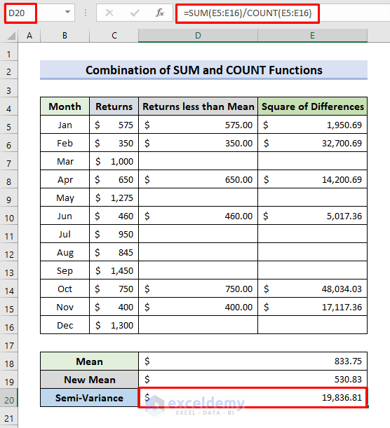
Spreadsheets are also commonly used for this calculation. The image below shows the same logic applied in Excel. The formula in cell D20 calculates the semi-variance by first identifying returns less than the mean (Column C), calculating their squared differences from the mean (Column E), and then averaging these squared differences.

3. Shortfall Probability: The Chance of Falling Short

While semi-variance measures the magnitude of downside risk, shortfall probability offers a more direct answer to a crucial question: "What is the probability that my return will be less than my minimum acceptable return?"

This minimum acceptable return is called the threshold return, denoted $R_L$. Shortfall risk is the risk of falling below this threshold, and the shortfall probability is simply $P(R<R_L)$.

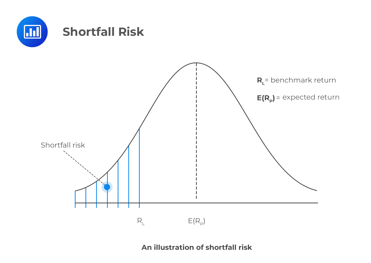
For discrete return distributions, calculating this is straightforward: you just sum the probabilities of all outcomes where the return is below $R_L$. For continuous distributions, like the normal distribution, we can use a clever tool called the Safety-First Ratio (SFRatio), developed by A.D. Roy.

The following reading explains this concept and its application.

The key insight from the reading is Roy's safety-first criterion: the optimal portfolio is the one that minimizes the probability of falling short of the threshold return. If returns are normally distributed, this is equivalent to choosing the portfolio with the highest Safety-First Ratio.

The formula is:

Where $E(R_p)$ is the portfolio's expected return, $R_L$ is the threshold return, and ${\sigma }_p$ is the portfolio's standard deviation. This ratio measures the "excess return" above the threshold per unit of risk.

As your statistics background suggests, this ratio is a z-score. The shortfall probability is then found using the cumulative distribution function (CDF) of the standard normal distribution, $\Phi$:

Your Turn: An Exam-Style Problem

Let's apply these concepts to a problem typical of the CM2 exam. The following question is adapted from actuarial education materials.

An investor is choosing between three investments, A, B, and C, with the following discrete return distributions:

• Investment A: 40% chance of 10% return; 20% chance of 15%; 40% chance of 20%.
• Investment B: 25% chance of 10% return; 70% chance of 15%; 5% chance of 40%.
• Investment C: A uniform distribution on the range [10%, 20%].

For Investment A and Investment B, try to calculate the following:

1. Expected Return: $E[R]$
2. Variance of Return: ${\sigma }^2(R)$
3. Semi-variance: Use the expected return you calculated in part 1 as the benchmark.
4. Shortfall Probability: Calculate the probability of the return being below 15%.

For Investment C, think about how you would approach these calculations for a continuous uniform distribution. What would be its expected return and variance?

Take some time to work through these calculations. This exercise directly applies the formulas and concepts we've covered today.

Conclusion

In this lesson, we have added three objective, statistical risk measures to our analytical toolkit. You are now equipped to calculate and interpret them, moving beyond subjective preferences to the hard data of return distributions.

Here are the key takeaways:

• Variance measures the total dispersion of returns around the mean, treating upside and downside volatility equally.
• Semi-variance improves upon variance by focusing only on downside risk—the squared deviations of returns that fall below a specified benchmark.
• Shortfall Probability provides the direct probability that an investment's return will fall short of a minimum acceptable threshold, $R_L$. For normally distributed returns, the Safety-First Ratio is a key tool for comparing portfolios and finding this probability.

In our next lesson, we will continue our focus on downside risk by exploring one of the most widely used risk measures in the financial industry: Value at Risk (VaR). We will define VaR, learn how to compute it for different distributions, and prepare to compare it with our final risk measure, Expected Shortfall.