Risk and Utility: Certainty Equivalent and Risk Premium

1. Defining the Certainty Equivalent and Risk Premium

In our last lesson, we saw that for a risk-averse person, the utility they get from the expected value of a gamble is greater than the expected utility of the gamble itself ($U(E[W])>E[U(W)]$). This creates a "gap" that reflects their dislike of risk. The certainty equivalent and risk premium are what give this gap a name and a number.

• The Certainty Equivalent (CE) is the amount of guaranteed money that would give an individual the same level of utility as a particular risky gamble. In other words, it's the risk-free cash amount that an investor would find equally attractive as the gamble. An investor would be indifferent between taking the gamble and receiving the certainty equivalent for sure. It is the answer to the question: "What is this gamble worth to you, in certain dollars?"

• The Risk Premium (RP) is the difference between the expected monetary value of a gamble and its certainty equivalent. It represents the amount of expected return an investor is willing to sacrifice to avoid the risk of the gamble. It answers the question: "How much are you willing to 'pay' out of the gamble's expected profit to get a sure thing instead?"

The relationship is:

For a risk-averse investor, the risk premium is always positive.

The following diagram provides a perfect visual summary of these concepts.

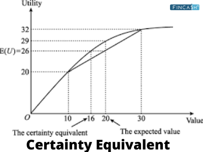
As the graph illustrates, we start with a gamble, find its expected utility $E(U)$, and then find the certain wealth level that gives us that exact same utility. That wealth level is the certainty equivalent.

2. The Calculation Process

The calculation follows a clear, three-step process that builds on what you already know.

1. Calculate the Expected Utility of the Gamble: This is exactly what we did in the last lesson. For a gamble with outcomes $W_i$ and probabilities $p_i$: $$E[U(W)]=\sum p_{i}U(W_i)$$
2. Find the Certainty Equivalent (C): By definition, the utility of the certainty equivalent is equal to the expected utility of the gamble. $$U(C)=E[U(W)]$$ To find $C$, you simply apply the inverse utility function, $U^{-1}$, to the expected utility value. $$C=U^{-1}(E[U(W)])$$
3. Calculate the Risk Premium (RP): First, calculate the expected monetary value of the gamble, $E[W]=\sum p_i{W}_i$. Then, use the definition of the risk premium. $$RP=E[W]-C$$

Let's watch a video that walks through this entire process with a numerical example using a square root utility function, which is a form of power utility ($U(W)=W^{0.5}$).

3. Examples with Key Utility Functions

Now, let's apply this method to the three key utility functions specified in the learning outcome.

Power Utility: $U(W)=\sqrt{W}$

The video you just watched used a square root utility function. For written reinforcement, the following resource works through another concise, numerical problem. This is a common format for exam questions.

Logarithmic Utility: $U(W)=\ln (W)$

Log utility functions are a cornerstone of financial modeling and represent a risk-averse investor with decreasing absolute risk aversion (meaning they are willing to risk more dollars as they get wealthier).

To solve for the certainty equivalent $C$ from the equation $\ln (C)=E[U(W)]$, you use the exponential function: $C=e^{E[U(W)]}$.

The following short video provides a very clear and quick numerical example of this calculation.

Exponential Utility: $U(W)=1-e^{-\alpha W}$

Exponential utility represents an investor with constant absolute risk aversion (CARA). This means their willingness to take a risk of a certain dollar amount doesn't change with their level of wealth. The parameter $\alpha >0$ determines the degree of risk aversion. (Note: sometimes the form $U(W)=-e^{-\alpha W}$ is used; the results for CE and RP are identical).

Let's work through an example together.
An investor has a utility function $U(W)=1-e^{-0.05W}$ and faces a gamble with a 50% chance of a final wealth of $50 and a 50% chance of a final wealth of $100.

1. Calculate Expected Utility $E[U(W)]$:
The utilities of the two outcomes are:

• $U(50)=1-e^{-0.05\times 50}=1-e^{-2.5}\approx 1-0.0821=0.9179$
• $U(100)=1-e^{-0.05\times 100}=1-e^{-5}\approx 1-0.0067=0.9933$

The expected utility is:

2. Find the Certainty Equivalent (C):
We set $U(C)$ equal to the expected utility:

Now, we solve for C:

The certainty equivalent of this gamble is approximately $62.28.

3. Calculate the Risk Premium (RP):
First, find the expected monetary value of the gamble:

Now, calculate the risk premium:

This investor is willing to give up $12.72 in expected value to avoid the risk of this gamble.

Conclusion

In this lesson, we have translated the abstract concept of risk aversion into concrete, calculable numbers that have real-world meaning for investment decisions. You now have the tools to quantify the value of a risky prospect for a given investor.

Here are the key takeaways:

• The Certainty Equivalent (C) is the risk-free amount that provides the same utility as a gamble. It's found by inverting the expected utility: $C=U^{-1}(E[U(W)])$.
• The Risk Premium (RP) is the compensation an investor demands for bearing risk. It's calculated as the difference between the gamble's expected monetary outcome and its certainty equivalent: $RP=E[W]-C$.
• For any risk-averse investor (concave utility function), the certainty equivalent will be less than the expected value of the gamble, resulting in a positive risk premium.
• You can now apply this three-step calculation process to gambles involving power, logarithmic, and exponential utility functions.

We have now explored how to model an investor's subjective attitude towards risk. In our next lesson, we will shift focus to objective, statistical measures used to quantify the risk inherent in an asset or portfolio, such as variance, semi-variance, and shortfall probability.