Expected Shortfall: Definition and Calculation

1. Defining Expected Shortfall

Expected Shortfall is the average of all potential losses that exceed the Value at Risk threshold. From a statistical perspective, it is a conditional expectation. It answers the question: "Given that we have experienced a loss greater than our VaR, what is our expected loss?"

The mathematical definition is:

where $L$ is the random variable representing loss, and $\alpha$ is the confidence level (e.g., 95% or 99%).

The following video provides an excellent conceptual introduction, recapping the limitation of VaR and clearly defining ES as the average of the tail losses.

The image below provides a powerful visual representation. While VaR is the single point marking the beginning of the tail, ES is the average value of all outcomes within that tail.

For most practical purposes, particularly in the context of the CM2 exam, Expected Shortfall (ES) and Conditional VaR (CVaR) are used synonymously. However, there is a subtle technical difference that is useful to know. ES is defined by a probability threshold (e.g., the average of the worst 5% of outcomes), whereas CVaR is strictly the average of losses given they exceed the VaR quantile. In continuous distributions, they are identical. In discrete distributions, where the VaR quantile can be ambiguous, ES provides a clearer, unambiguous measure.

2. Computing Expected Shortfall

Just as with VaR, we can compute ES using historical data or by assuming a parametric distribution.

Method 1: Historical Simulation

This method is the most intuitive. It follows directly from the definition of ES as an average of tail losses. The steps are:

1. Gather a set of historical or simulated profit/loss observations.
2. Sort the observations from largest profit to worst loss.
3. Determine the VaR cutoff point. For example, with 100 observations and a 95% confidence level, the tail consists of the 5 worst losses. The 95% VaR would be the 5th worst loss.
4. Calculate the average of all losses that are worse than or equal to the VaR. This average is the Expected Shortfall.

The following video provides a detailed, step-by-step numerical calculation that makes this process very clear.

As you saw in the video, for a 95% confidence level with 100 observations, the ES is the average of the 5 worst losses. For a 97% confidence level, it's the average of the 3 worst losses. It's a straightforward conditional average.

Method 2: The Parametric (Normal) Method

When we assume that losses (or returns) follow a normal distribution, we can use a specific formula to calculate ES. This bypasses the need for sorting large datasets and relies on the distribution's parameters.

For a loss distribution $L\sim N({\mu }_L,{\sigma }_L^2)$, the Expected Shortfall at a confidence level $\alpha$ is given by:

where:

• ${\mu }_L$ is the mean of the loss distribution.
• ${\sigma }_L$ is the standard deviation of the loss distribution.
• $z_{\alpha }$ is the standard normal quantile for the confidence level $\alpha$ (e.g., for $\alpha =95\%$, $z_{0.95}=1.645$).
• $\varphi (\cdot )$ is the probability density function (PDF) of the standard normal distribution.
• $1-\alpha$ is the significance level of the tail (e.g., 5% or 0.05).

The video you just watched also covers this.

This formula is very powerful. Since you have a strong background in probability, you can appreciate that it elegantly combines the distribution's parameters ($\mu$, $\sigma$) with the properties of the normal curve ($\varphi$, $z$) to derive the conditional expectation in the tail.

Your Turn: Calculating ES

Let's apply the historical simulation method to a small dataset. This will solidify your understanding of the core computation.

Problem:
A portfolio has generated the following 20 daily losses over the past month, sorted from best outcome (a gain) to worst loss (in thousands of dollars):
[-5, 2, 8, 10, 15, 17, 20, 22, 24, 25, 28, 30, 31, 33, 35, 40, 42, 50, 65, 80]

Calculate the 90% VaR and the 90% ES for this portfolio.

Solution Steps:

1. Determine the number of observations in the tail. The confidence level is 90%, so the tail is the worst $100\%-90\%=10\%$ of outcomes.
   Number of tail observations = $10\%\times 20=2$.
2. Identify the VaR. The 90% VaR is the loss at the cutoff point, which is the 2nd worst loss. Looking at the sorted list, the worst loss is 80 and the second worst is 65. So, the 90% VaR is $65,000.
3. Calculate the Expected Shortfall. The 90% ES is the average of all losses in the 10% tail. In this case, it's the average of the two worst losses.
   ES = $\frac{80+65}{2}=\frac{145}{2}=72.5$.
   So, the 90% ES is $72,500.

Notice that ES ($72.5k) is greater than VaR ($65k), which must always be the case.

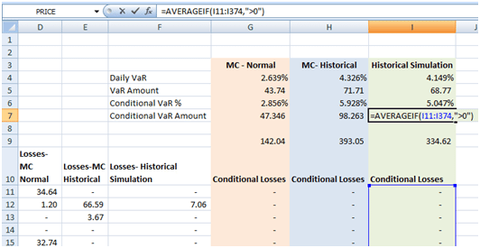
The image below from a spreadsheet calculation shows a similar logic for a different dataset, calculating CVaR (ES) by averaging the losses in the tail.

Conclusion

In this lesson, we have moved beyond VaR to a more informative measure of tail risk. Expected Shortfall gives us a crucial piece of information that VaR omits: the expected magnitude of our losses when we venture into the tail of the distribution.

Here are the key takeaways:

• Expected Shortfall (ES), or Conditional VaR (CVaR), is the expected loss conditional on that loss exceeding the VaR. It answers, "How bad can losses get on average in a worst-case scenario?"
• It is calculated by averaging all losses in the tail of the distribution beyond the VaR quantile.
• For historical data, this involves identifying the worst $(1-\alpha )\%$ of outcomes and calculating their average.
• For a normal distribution, a specific formula involving the distribution's mean, standard deviation, and the normal PDF is used.
• By definition, ES will always be greater than or equal to VaR.

While we have now defined both VaR and ES and know how to compute them, we haven't formally discussed why ES is considered a "better" risk measure from a theoretical standpoint. In our next lesson, we will delve into the mathematical properties of risk measures and explore the concept of coherence. We will see why ES satisfies these desirable properties, particularly subadditivity, while VaR does not.