Lorentz Force and Thermal Stress Simulation

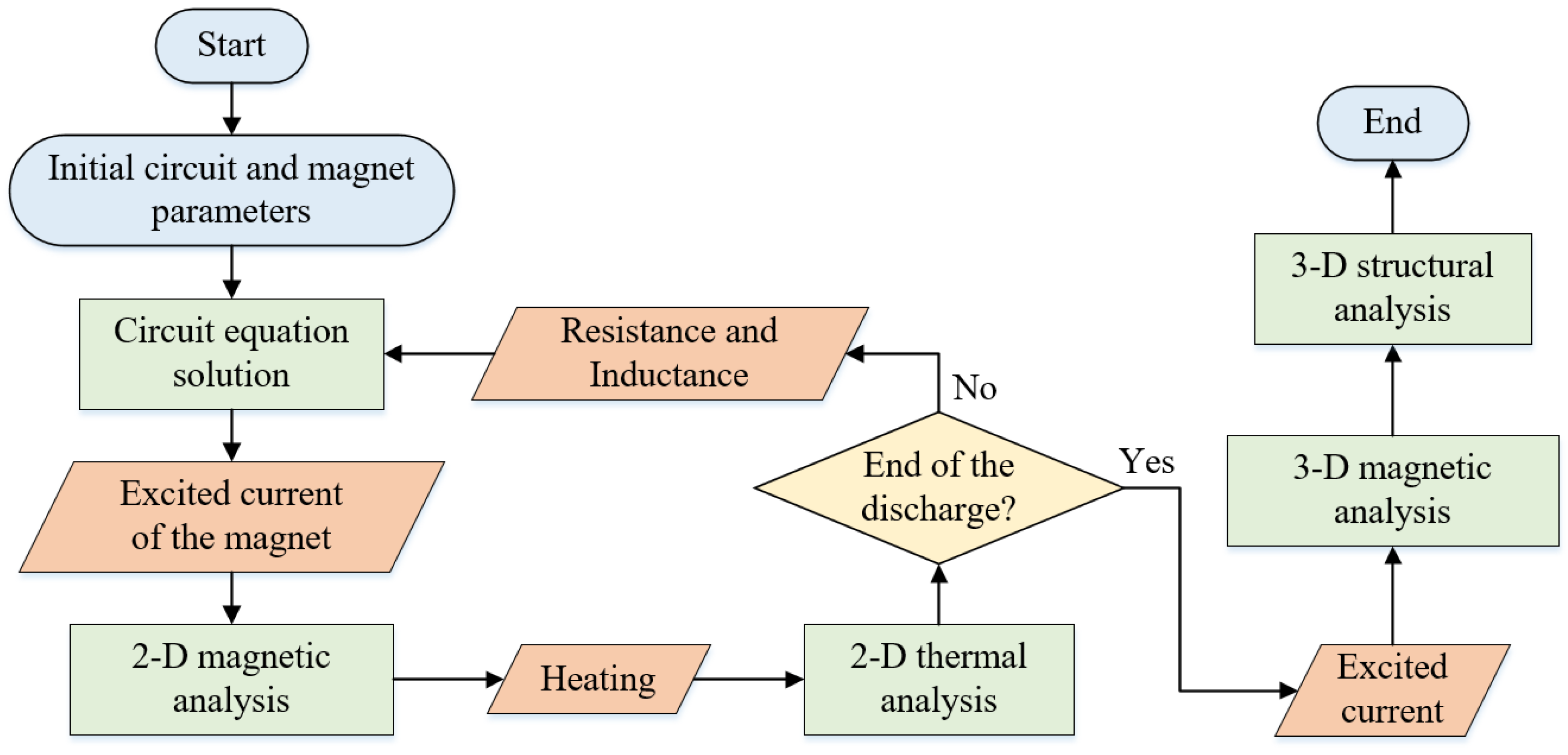
1. From Physics to Mechanical Loads

A structural simulation requires "loads"—the forces and effects that cause the object to deform. For a pulsed magnet, these loads come directly from the electromagnetic and thermal physics we've already studied.

Lorentz Forces

The primary load is the Lorentz force, generated by the interaction of the current in the windings with the magnetic field. The force density ${\vec{f}}_L$ (force per unit volume) is given by:

In a solenoid, this force is directed radially outwards and axially inwards (compressing the coil), generating immense pressure. In a Finite Element Method (FEM) simulation, this is not applied as a simple external force but as a body force, a force that acts on the entire volume of the conducting elements. The software first solves for $\vec{B}(\vec{r},t)$ from $\vec{J}(\vec{r},t)$ and then uses both to compute the force field ${\vec{f}}_L(\vec{r},t)$ at every point within the conductor for each time step.

Thermal Expansion

The second major load is thermal expansion. As the coil heats up from Joule losses, the material expands. The resulting thermal strain, ${ϵ}_{th}$, for an isotropic material is:

where $\alpha (T)$ is the temperature-dependent coefficient of thermal expansion and $T_{ref}$ is the initial, stress-free temperature. This effect is critical. The inner windings heat up the most and want to expand, but they are confined by the cooler, outer reinforcement layers. This mismatch in expansion creates significant internal stresses, which are superimposed on the stresses from the Lorentz force.

2. Describing Large Deformations: A Deeper Look at Strain

In your introductory mechanics courses, you encountered strain as $ϵ=\Delta L/L$. This is the infinitesimal strain tensor, which is only accurate for very small deformations and rotations. Given that pulsed magnets can experience significant plastic deformation, a more robust framework is needed for accurate modeling. Your physics and math background will be useful for appreciating this more rigorous approach.

To properly describe how a material deforms, continuum mechanics introduces the deformation gradient tensor, $F$. It relates a vector in the undeformed material to its new orientation and length in the deformed material. A key insight is that $F$ contains information about both pure deformation (stretching/shearing) and rigid body rotation. To isolate the pure deformation, we use a polar decomposition:

Here, $R$ is a rotation matrix and $U$ is the symmetric right stretch tensor, which purely describes the stretching of the material.

From this, we can define strain tensors that are suitable for large deformations. One of the most important is the Green-Lagrange strain tensor, $E$:

where $I$ is the identity tensor. The key properties of $E$ are:

• It is zero for any rigid body motion (translation or rotation), making it a pure measure of deformation.
• For small deformations, it reduces to the familiar infinitesimal strain tensor.

To solidify these concepts, which are fundamental to the algorithms used in FEM solvers, please watch the following video.

This theoretical foundation is what allows FEM software to accurately calculate strains and, consequently, stresses, even when the magnet coil is pushed into plastic deformation.

3. A Practical Guide to Structural Simulation

Let's now walk through the process of setting up a structural simulation for a pulsed magnet coil. We will use the detailed technical report by M.G.N.M. Oudendijk, which analyzes a high-field magnet using the MARC finite element program, as our guide. The principles discussed are applicable to any modern FEM package.

Step 1: Discretization and Geometry (Section 3.2)

The first step is to create a model. Given the cylindrical nature of a solenoid, an axisymmetric 2D model is often sufficient and computationally much cheaper than a full 3D model.

• The model represents a cross-section of the coil.
• Symmetry about the mid-plane is used, so only half of the cross-section is needed.
• The mesh is refined in areas where high stress gradients are expected (e.g., near the inner bore).

This is Figure 3.2.1 from the Oudendijk report, showing the axisymmetric mesh of a single coil. Note the symmetry about the mid-plane and the axis of rotation.

Step 2: Material Modeling (Section 3.3)

This is the most complex part. A coil is not a monolithic object; it's a composite of conductor (e.g., copper) and insulation (e.g., epoxy resin).

• Composite Behavior: The report describes a sophisticated method where the elastic properties of the winding/insulation composite are calculated using models like Halpin-Tsai.
• Plasticity: Plastic deformation is assumed to be dominated by the conductor. To check for this, the stresses in the winding material are calculated from the overall composite stresses.
• Yield Criterion: Plasticity begins when the stress state reaches a critical level. This is determined by a yield criterion. The most common for metals is the von Mises yield criterion. It combines the different stress components into a single equivalent stress, ${\sigma }_{vM}$. The material yields when ${\sigma }_{vM}$ exceeds the material's yield strength, ${\sigma }_{yield}$. $${\sigma }_{vM}=\sqrt{{\sigma }_{xx}^2+{\sigma }_{yy}^2+{\sigma }_{zz}^2-({\sigma }_{xx}{\sigma }_{yy}+{\sigma }_{yy}{\sigma }_{zz}+{\sigma }_{zz}{\sigma }_{xx})+3({\sigma }_{xy}^2+{\sigma }_{yz}^2+{\sigma }_{zx}^2)}$$

Step 3: Loads and Boundary Conditions (Section 3.3)

• Boundary Conditions: An axial displacement of zero is enforced at the mid-plane due to symmetry.
• Loads: The Lorentz forces are applied as body forces, scaled by the fraction of conductor in each element. The thermal load is applied by defining the temperature of the elements from the thermal simulation.

Step 4: Analyzing the Results (Section 3.4)

The simulation's output is a rich dataset of stress and strain tensors at every point in the model.

• Stress Components: We can plot individual components like tangential (hoop) stress, radial stress, and axial stress.
• Equivalent Stress: The von Mises stress is plotted to see which regions of the coil have yielded (i.e., where ${\sigma }_{vM}\ge {\sigma }_{yield}$).
• Deformation: We can visualize how the coil shape changes under load.

Let's examine some typical results. The figures below, from the Oudendijk report and another study, show the calculated stress distribution and resulting deformation.

Figure 3.4.1 from the Oudendijk report. It shows the calculated stress components in the mid-plane at maximum field (a) and the residual stresses after the pulse (b). Notice the high tangential (hoop) stress and compressive radial stress.

4. Coupling Thermal and Mechanical Effects

Now we combine everything. The total strain ${ϵ}_{total}$ at any point is the sum of the elastic strain ${ϵ}_{elastic}$, plastic strain ${ϵ}_{plastic}$, and thermal strain ${ϵ}_{thermal}$. The structural solver must account for all of these simultaneously.

Section 3.7.3 of the Oudendijk report investigates exactly this coupling for a steel-reinforced coil.

• The winding material heats up and tries to expand (${ϵ}_{thermal}$).
• The massive steel reinforcement remains much cooler and does not expand as much.
• The result is a significant increase in the compressive radial stress between the coil and the shield. The hot coil pushes outwards against the cold shield.

This is a perfect example of a coupled multi-physics problem where thermal expansion and Lorentz forces combine to determine the final stress state. A real-world example is seen in the "Foil Coil" paper, which uses FEA to visualize this stress transfer.

The FEA images in this paper (Figure 3) clearly show how the internal forces are transmitted through the copper foil and into the external reinforcement, providing a tangible example of the stress distributions we've been discussing.

Conclusion

You have now completed the full multi-physics simulation chain for designing a pulsed magnet. We started with the electrical circuit, moved to the magnetic and thermal fields, and have now used those results to perform a structural analysis.

Key Takeaways:

• Structural simulations of pulsed magnets are driven by two primary loads: Lorentz forces (applied as body forces) and thermal expansion (applied as an initial strain).
• For accurate analysis of large deformations, advanced strain measures like the Green-Lagrange tensor are used, which are rotationally invariant.
• Practical FEM modeling involves simplifying the geometry (e.g., axisymmetry) and using sophisticated material models that account for the composite nature of the coil and plastic deformation (e.g., via the von Mises yield criterion).
• The output of the simulation provides detailed stress and strain distributions, allowing engineers to identify high-stress regions and assess whether the magnet will survive the pulse.

Next Lesson Preview:
So far, our simulations have been for analysis—predicting the performance of a given design. The next step is to use this predictive power for synthesis—creating a better design. In the next lesson, we will learn how to formulate a design optimization problem with a clear objective function and constraints. We will explore how to use algorithms to automatically search for an optimal coil geometry that maximizes performance (like the central field) while respecting physical limits (like the maximum allowable stress).