Coupled Electromagnetic-Thermal Simulation of Coil Pulse Heating

1. The Physics of Multi-Physics Coupling

At its heart, a coupled electromagnetic-thermal simulation solves two sets of physical laws simultaneously and allows them to influence each other. Your background in physics and mathematics will make the governing equations familiar.

• Electromagnetics: Maxwell's equations, solved in a transient form, determine the evolution of the current density $\vec{J}(\vec{r},t)$ throughout the conductor.
• Thermodynamics: The heat diffusion equation governs the temperature distribution $T(\vec{r},t)$: $${\rho }_m{c}_p\frac{\partial T}{\partial t}+\nabla \cdot (-k\nabla T)=Q$$ where ${\rho }_m$ is the mass density, $c_p$ is the specific heat capacity, $k$ is the thermal conductivity, and $Q$ is the volumetric heat source.

The Coupling Mechanism:

The two physics domains are not independent. They are linked through two critical relationships that form an iterative feedback loop, as illustrated in the flowchart below.

1. Electromagnetics $\to$ Thermal (The Heat Source): The current flowing through the resistive conductor generates Joule heat. This becomes the source term $Q$ in the heat equation:

   $$Q(\vec{r},t)=\vec{E}\cdot \vec{J}={\rho }_{el}|\vec{J}(\vec{r},t){|}^2$$

   where ${\rho }_{el}$ is the electrical resistivity.

2. Thermal $\to$ Electromagnetics (The Feedback): The temperature change is not just a result; it's an input. The material properties of the conductor, most importantly its electrical resistivity (${\rho }_{el}$), but also its thermal conductivity ($k$) and specific heat capacity ($c_p$), are strong functions of temperature.

   $${\rho }_{el}={\rho }_{el}(T),k=k(T),c_p=c_p(T)$$

   As the coil heats up, its resistance increases. For a given circuit, this changes the current pulse itself, typically damping it more strongly. The FEM solver accounts for this at each time step, creating a fully coupled, dynamic simulation.

2. A Practical Guide to Setting Up a Coupled Simulation

Let's translate this theory into the practical steps you would take in a commercial FEM package like COMSOL Multiphysics. The following video demonstrates a coupled simulation for induction heating. While the application is different, the core physics—an electromagnetic field generating heat in a conductor—and the software workflow are identical to what's needed for a pulsed magnet.

This walkthrough gives you a concrete mental model of the entire process, from defining the problem to visualizing the results.

3. Application to Pulsed Magnets: A Case Study

Now, let's connect this general workflow to the specific case of a pulsed magnet. The current in a capacitor-driven magnet isn't a steady sinusoid; it's a transient pulse, typically a damped sine wave.

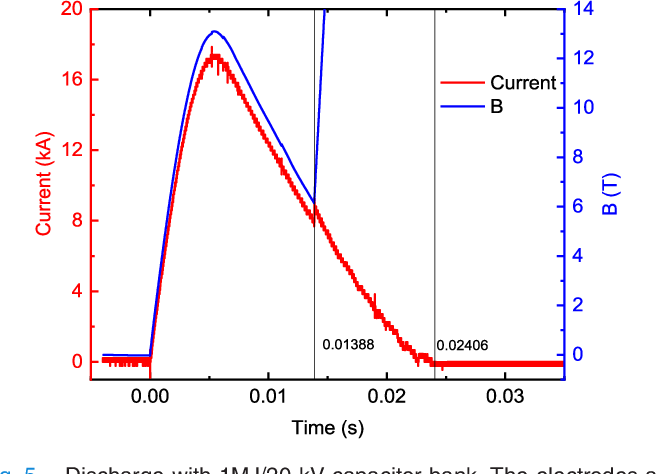
A research paper analyzing thermodynamic processes in a wire-wound pulsed coil provides an excellent example of the results of such a coupled simulation. While they used a different tool (MATLAB/Simulink), the physical model is the same.

This paper perfectly encapsulates the "why" behind this lesson. The coupled simulation isn't just a complex academic exercise; it's a predictive tool essential for understanding and optimizing the real-world performance of a pulsed magnet.

4. Advanced Models and Validation

The principles we've discussed scale to even more complex systems. For instance, high-temperature superconductor (HTS) magnets involve tapes with multiple layers (superconductor, copper, substrate, etc.). Simulating a quench (the transition from superconducting to normal resistive state) requires an even more detailed model.

The paper "Electromagnetic-thermal finite element model coupled to..." (Resource ID: LINK), which you can look at for further insight, details such a model. Its Figure 6 provides a sophisticated view of the TEFEM-ECM (Thermo-Electro-Magnetic Finite Element Model coupled to an Electrical Circuit Model). It shows how currents are redistributed among the different layers of an HTS tape as the temperature rises during a pulse, a phenomenon known as current sharing. The paper's ultimate goal, as seen in its Figures 16 through 21, is to compare simulation outputs (current, voltage, temperature) with real experimental data, reinforcing the critical role of experimental validation.

Conclusion

Today, we've added a critical layer of physics to our simulation toolkit. You now understand the principles and practical steps for creating a coupled simulation that predicts the thermal evolution of a coil during a pulse.

Key Takeaways:

• Coupled electromagnetic-thermal simulations are essential for predicting temperature rise and its impact on pulsed magnet performance.
• The simulation is built on a feedback loop: $\vec{J}$ generates heat $Q$, and the resulting temperature $T$ changes the material properties (especially ${\rho }_{el}$), which in turn affects $\vec{J}$.
• The practical workflow involves using a coupled physics interface, defining temperature-dependent material properties using interpolation tables, and running a transient (time-dependent) study.
• The results of such simulations provide crucial design insights, predicting the peak temperature, the reduction in peak field due to heating, and allowing for validation against experimental data.

Next Lesson Preview:
We have now mastered the calculation of $\vec{J}(\vec{r},t)$, $\vec{B}(\vec{r},t)$, and $T(\vec{r},t)$. This completes the electromagnetic and thermal analysis. What's next? The immense forces and temperature gradients generate mechanical stress. In our next lesson, we will perform a structural mechanics simulation to calculate stress and strain distributions from Lorentz forces and thermal expansion, adding the final piece to our multi-physics model.