FEM Fundamentals for Coupled Multi-Physics in Magnet Design

1. The Core Idea: Divide and Conquer

At its heart, the Finite Element Method is a powerful numerical technique for finding approximate solutions to partial differential equations (PDEs). The fundamental idea is to replace a complex, continuous problem domain with a collection of smaller, simpler, interconnected subdomains called finite elements.

Instead of trying to solve the governing equations (like Maxwell's equations or the heat equation) over the entire, complex geometry at once, we solve a simplified version of the problem on each small element and then "stitch" the solutions together.

To get a clear visual and conceptual overview of this process, let's watch a video from The Efficient Engineer.

Let's summarize the key ideas from the video:

• Discretization: The continuous physical domain of our magnet—the windings, reinforcement, bore, etc.—is broken down into a finite number of elements. The collection of all these elements and their connection points (nodes) is called the mesh.
• Element Types: Depending on the problem's dimensionality and geometry, we can use 1D line elements, 2D surface elements (triangles, quadrilaterals), or 3D solid elements (tetrahedra, hexahedra).
• Degrees of Freedom (DOFs): For each node, we define the physical quantities we want to determine. In a structural analysis, this would be displacements and rotations. In a thermal analysis, it's temperature. In an electromagnetic analysis, it's often the magnetic vector potential. The goal of an FEM simulation is to compute the values of these DOFs at every node in the mesh.

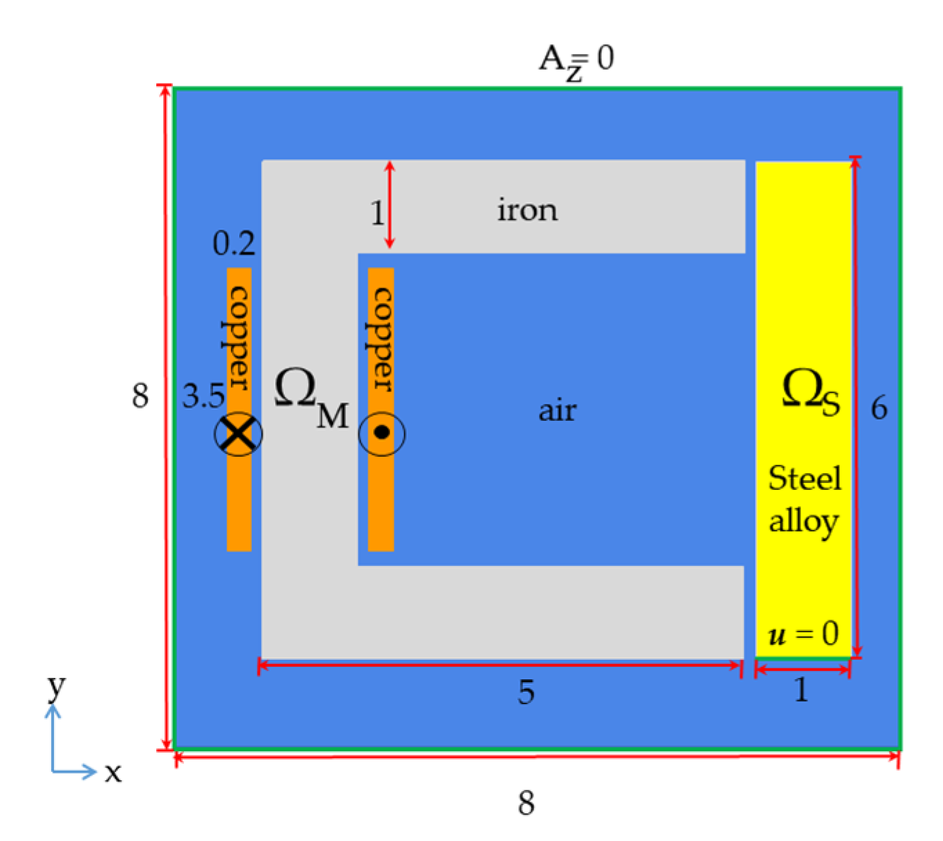
2. The Mathematical Engine of FEM

Now that we have the conceptual framework, let's delve into how FEM translates a physics problem described by a PDE into a system of algebraic equations that a computer can solve. Your background in physics and mathematics will be very helpful here, as the method is rooted in concepts from vector calculus and linear algebra.

The process involves transforming the PDE, known as the strong form of the problem, into an equivalent integral equation, called the weak form. This step is crucial because the weak form is more forgiving about the smoothness of the solution and is much better suited for numerical approximation.

The following video provides a clear, step-by-step derivation for a 1D problem, which beautifully illustrates the core mathematical principles that apply to more complex 2D and 3D problems.

Let's break down that dense but critical process:

1. From Strong to Weak Form: We start with the governing PDE (e.g., Poisson's equation ${\nabla }^{2}u=f$). This is the "strong form" because it must hold true at every single point in the domain. We multiply the entire equation by an arbitrary "test function" $v$ and integrate over the domain. Using integration by parts (or the divergence theorem in higher dimensions), we shift a derivative from our unknown function $u$ to the test function $v$. The result is an integral equation, the "weak form," which is equivalent to the original PDE but imposes less strict continuity requirements on the solution $u$.

2. Discretization with Shape Functions: We can't find the exact continuous function $u$, so we approximate it. Within each element, we approximate $u$ as a linear combination of simple, predefined polynomials called shape functions (or basis functions), $N_i$. The coefficients of this combination are the unknown nodal values (the DOFs), $u_i$. For example, inside one element, the approximate solution $\tilde{u}(x)$ might be $\tilde{u}(x)=N_1(x)u_1+N_2(x)u_2$. The shape functions interpolate the solution between the nodes.

3. Assembly of Linear Equations: We substitute this approximate solution into the weak form. Since the weak form must hold for any valid test function $v$, this leads to a system of linear algebraic equations. This system is famously written as:

   $$[K]\{U\}=\{F\}$$

   where:

   • $\{U\}$ is the global vector of unknown nodal values (the DOFs) for the entire mesh. This is what we want to solve for.
   • $[K]$ is the global stiffness matrix (the name comes from its origins in structural mechanics). It represents the physical properties of the system (e.g., material conductivity, elastic modulus) and the geometry of the mesh. It's assembled by calculating a smaller "element stiffness matrix" for each element and then adding them together based on how the elements are connected.
   • $\{F\}$ is the global force vector, which represents the external loads or sources applied to the system (e.g., applied currents, heat sources, external pressures).

4. Solving the System: After applying boundary conditions (e.g., fixing the potential on a conductor or the temperature on a cooled surface), this large system of linear equations is solved by the computer using efficient numerical linear algebra algorithms to find the unknown nodal values in $\{U\}$. From these nodal values, we can then calculate secondary quantities like magnetic field strength, stress, and strain anywhere in the domain.

3. Application to Magnet Design: Coupled Multi-Physics

Designing a high-field pulsed magnet is not just an electromagnetic problem. It's a classic coupled multi-physics problem where different physical domains strongly influence each other.

1. Electromagnetic (EM) Analysis: Solves Maxwell's equations (often in magnetic vector potential form) to find the magnetic field $B(t)$ and current density $J(t)$ throughout the coil during the pulse.

   • Output: This provides two critical inputs for the other physics domains:
     • Lorentz forces: ${\vec{F}}_L=\vec{J}\times \vec{B}$, which are the source of mechanical stress.
     • Joule heating: $Q=\int J(t{)}^2\rho dt$, which acts as a heat source.

2. Structural (Mechanical) Analysis: Solves the equations of solid mechanics to find the stress $\sigma$ and strain $ϵ$ in the coil.

   • Input: The Lorentz forces from the EM analysis and thermal expansion forces due to temperature changes from the thermal analysis.
   • Output: Determines if the coil will mechanically survive the pulse.

3. Thermal Analysis: Solves the heat diffusion equation to find the temperature distribution $T(t)$ in the coil during and after the pulse.

   • Input: The Joule heating from the EM analysis.
   • Output: Determines the peak temperature of the conductor and the required cooling time.

The key word here is coupled. The temperature rise from the thermal analysis changes the electrical resistivity $\rho$ and the mechanical properties (like Young's modulus) of the materials. This change in resistivity feeds back into the EM analysis, altering the current distribution and subsequent heating. This interdependency requires an iterative solution.

To handle this, FEM software typically employs a sequential, iterative approach. Let's look at a text that describes this process.

The flowchart in Figure 2.12a shows the essence of a weakly coupled multi-physics simulation:

1. Initial Guess: Start with an initial temperature (e.g., 77 K for an LN2-cooled coil).
2. EM Simulation: Run an FEM electromagnetic simulation to calculate the current, fields, Lorentz forces, and Joule heat generated during the pulse, using the material properties at the current temperature.
3. Thermal & Structural Simulation: Feed the calculated heat sources and forces into the thermal and structural FEM models.
4. Update Temperature: The thermal simulation calculates a new temperature distribution.
5. Check for Convergence: Compare the new temperature distribution to the one from the previous iteration. If they are sufficiently close, the solution has converged. If not, update the material properties (resistivity, etc.) based on the new temperature and go back to step 2.

This loop continues until a self-consistent solution is found where the electromagnetic, thermal, and mechanical states are all in equilibrium. This is precisely the process used in software like PMDS or commercial packages (ANSYS, COMSOL) to design and verify pulsed magnets.

Conclusion

In this lesson, we have opened the door to the modern numerical methods used to design high-field magnets. We moved from the "what" of magnet design to the "how."

Key Takeaways:

• The Finite Element Method (FEM) solves complex physics problems by discretizing the domain into a mesh of simple elements and solving a system of algebraic equations for unknown values (DOFs) at the element nodes.
• The mathematical core of FEM involves transforming the governing partial differential equation (strong form) into an equivalent integral equation (weak form), which is better suited for numerical approximation with simple shape functions.
• Magnet design is a coupled multi-physics problem where electromagnetic forces create mechanical stress, and Joule heating raises the temperature.
• FEM solves these coupled problems iteratively: the outputs of one physics simulation (e.g., heat from EM) become the inputs for another (e.g., thermal), in a loop that continues until a self-consistent solution is reached.

Next Lesson Preview:
Now that you understand the fundamental principles of what FEM is and how it handles coupled physics, we will move on to its practical application. In the next lesson, we will explore how specialized software packages use these principles to perform a key task in magnet design: calculating the magnetic field distribution in a complex coil geometry.