Joule Heating and Adiabatic Temperature Rise in Conductors

Hello! Welcome to your fourth lesson in the "Principles of Pulsed Field Generation" module.

In our last two lessons, we established how to determine a pulse's peak field from the stored energy ( $B_{p e ak} \propto E / L$ ) and its duration from the circuit parameters ( $τ \approx π L C$ ). We now have a good picture of the current pulse, $I (t)$ , flowing through the magnet coil. A natural and critical question follows: what are the consequences of forcing such a massive current through a resistive conductor?

The primary consequence is intense heating. This lesson is dedicated to understanding and quantifying this effect. Our learning outcome is to estimate the Joule heating and adiabatic temperature rise in a conductor during a single pulse. The temperature rise is one of the most fundamental limits in pulsed magnet design, as it affects material strength, insulation integrity, and ultimately, the magnet's survival.

1. The Adiabatic Approximation and Energy Balance

When a current pulse lasts for only tens of milliseconds, there is very little time for the generated heat to conduct away from the windings. The heating process is therefore very close to adiabatic. We can assume that all the electrical energy dissipated as heat is absorbed by the conductor itself, causing its temperature to rise.

To model this, let's consider a small volume element of the conductor. The electrical power dissipated as heat per unit volume is given by Joule's first law, expressed in terms of current density $j$ and resistivity $ρ$ :

$p_{g e n} = j \cdot E = j^{2} ρ$

This generated heat is absorbed by the material, increasing its internal energy and thus its temperature. The energy absorbed per unit volume to produce a temperature change $d T$ is:

$d q_{ab s} = D c d T$

where $D$ is the material's density and $c$ is its specific heat capacity.

Under the adiabatic assumption, we can equate the heat generated in a time interval $d t$ with the heat absorbed:

$j (t)^{2} ρ (T) d t = D c (T) d T$

Notice that we've explicitly written resistivity and specific heat as functions of temperature, $ρ (T)$ and $c (T)$ . This is crucial, as these properties can change significantly over the temperature range of a pulse (e.g., from 77 K to 400 K). This energy balance equation is the foundation for our analysis.

2. The Action Integral and Material Function

To find the total temperature rise over a whole pulse, we need to integrate the energy balance equation. We can separate the time-dependent and temperature-dependent variables:

$\int_{t_{i}}^{t_{f}} j (t)^{2} d t = \int_{T_{i}}^{T_{f}} \frac{D c ( T )}{ρ ( T )} d T$

This elegant result separates the problem into two distinct parts:

The Action Integral: The left-hand side, $\int j (t)^{2} d t$ , depends only on the current pulse's shape and magnitude. It represents the total thermal load imposed on the conductor by the pulse.
The Material Integral: The right-hand side depends only on the material properties and the initial and final temperatures. It quantifies the material's ability to absorb thermal energy.

This powerful framework is central to pulsed magnet design. For a more detailed look at this derivation and its application, we'll turn to a key reference.

Design and Optimization of Force-Reduced High Field ...

The dissertation 'Design and Optimization of Force-Reduced High Field ...' by Szabolcs Rembeczki provides an excellent and detailed derivation of the thermal analysis for pulsed coils. It formalizes the concepts we've just introduced.

Please read sections 5.5.1 ('Heat Analysis and Coil Cooling') and 5.5.2 ('Action Integral'). In 5.5.1, focus on the setup of the energy balance equation. In 5.5.2, pay close attention to the definitions of the 'action integral' and 'material integral' F_{mat}. Observe how the action integral is simplified for different pulse shapes using the parameter \xi, and how this leads to the final equation for the maximum current density, j_0.

As the text explains, we can write the action integral as $\int j (t)^{2} d t = j_{0}^{2} τ ξ$ , where $j_{0}$ is the peak current density, $τ$ is the pulse duration, and $ξ$ is a pulse shape factor.

For a half-sine pulse, $ξ = 1/2$ .
For a rectangular pulse, $ξ = 1$ .
For a triangular pulse, $ξ = 1/3$ .

This allows us to express the peak current density that a conductor can handle for a given temperature rise ( $T_{i} \to T_{f}$ ) and pulse profile ( $τ, ξ$ ):

$j_{0} = \frac{F _{ma t} ( T _{i} , T _{f} )}{τ ξ}$

where $F_{ma t} (T_{i}, T_{f}) = \int_{T_{i}}^{T_{f}} \frac{D c ( T )}{ρ ( T )} d T$ .

This equation is a cornerstone of pulsed magnet design. It tells you that for a longer pulse (larger $τ$ ) or a "fatter" pulse (larger $ξ$ ), the maximum allowable peak current density $j_{0}$ decreases, assuming the material and temperature limits are fixed.

3. A Refinement: The Effect of Magnetoresistance

Your physics background in condensed matter will tell you that a material's resistivity doesn't just depend on temperature. In a high-field magnet, we must also consider magnetoresistance: the increase in resistance due to the magnetic field itself. The Lorentz force causes the charge carriers to follow curved paths between collisions, increasing their path length and thus the measured resistance.

This effect can be significant. The resistivity becomes a function of both temperature and field, $ρ (B, T)$ . This complicates our material integral, as $ρ$ now also varies during the pulse because $B$ is changing.

Design and Optimization of Force-Reduced High Field ...

Let's return to the same dissertation to see how this effect is incorporated.

Please read section 5.5.3 ('Effect of Magnetoresistance'). Note the empirical formula provided for the resistivity of copper as a function of both B and T. Look at Figure 5.27, which plots ( ho(T)) for different field strengths, and Figure 5.28, which shows how the maximum current density is reduced by the magnetic field. This is a crucial real-world correction to our simple model.

For a precise calculation, one would need to solve the coupled electro-thermo-magnetic problem, often numerically. For a first-order estimate, one can use the peak magnetic field $B_{p e ak}$ in the resistivity formula to get a conservative (i.e., higher) estimate of the final temperature.

4. From Theory to Practice

Let's see how these estimations play out in real-world magnets. The analysis often provides an average temperature rise, but local "hot spots" can be the real point of failure.

This image shows a simulation of temperature distribution in a coil during a pulse. Note that the heating is not uniform; it's concentrated in specific regions.

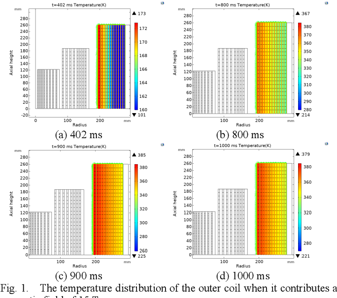
Temperature Distribution in a Pulsed Magnet Outer Coil Over Time — Simulated temperature distribution in Kelvin for the outer coil of a pulsed magnet at different times during the pulse. This illustrates the non-uniform Joule heating, with higher temperatures concentrated at the inner radius and ends of the coil.

A published paper on a novel magnet design gives us concrete numbers and a glimpse into how temperature is measured experimentally.

A novel pulsed magnet for magnetic linear birefringence ...

The paper 'A novel pulsed magnet for magnetic linear birefringence...' describes the design and testing of a 'Foil Coil' magnet. It provides valuable practical data on temperature rise.

Please read sections III.B ('Realization') and III.C ('Tests'). In III.B, notice the discussion about the holes in the copper foil. The reduced cross-section increases the local current density, leading to a local temperature rise that is twice as high. This is a perfect example of why j is more fundamental than I. In III.C, look at Figure 8 and the surrounding text. The authors estimate a temperature rise of 35 K for a 20 T pulse. Crucially, they describe how they deduce the coil's temperature by measuring its total resistance, using the known temperature dependence of copper's resistivity. This is a standard diagnostic technique.

The technique of measuring resistance to infer temperature is a direct application of the $ρ (T)$ relationship we've been discussing. By measuring the coil's resistance $R$ before a pulse (at a known temperature $T_{i}$ ) and immediately after (before it cools), one can determine the final average temperature $T_{f}$ .

Test your understanding!

A pulsed magnet coil is made of copper and pre-cooled to 77 K. It is subjected to a 15 ms half-sine pulse with a peak current density of $j_{0} = 4 \times 1 0^{9} A/m^{2}$ . Using the data from the resources, estimate the final temperature of the coil.

Hint: Use the plots from the Rembeczki dissertation (Resource LINK). You'll need to calculate the action integral first, then find the corresponding final temperature on the material integral plot.

Show answer

Calculate the Action Integral:
For a half-sine pulse, $ξ = 1/2$ . The pulse duration is $τ = 15 ms = 0.015 s$ .
The action integral is:
$\int j^{2} d t = j_{0}^{2} τ ξ = (4 \times 1 0^{9} A/m^{2})^{2} \times (0.015 s) \times (0.5)$
$\int j^{2} d t = (16 \times 1 0^{18}) \times (0.0075) = 1.2 \times 1 0^{17} A^{2} s / m^{4}$
Use the Material Integral Plot:
The action integral is equal to the material integral, $F_{ma t}$ . We need to find the final temperature $T_{f}$ that corresponds to this value. Let's look at Figure 5.24 from the dissertation.
We start on the curve for $T_{i} = 77 K$ . We find the value $1.2 \times 1 0^{17}$ on the y-axis (or $12 \times 1 0^{16}$ in the plot's units).
Following this value across to the $T_{i} = 77 K$ curve and then down to the x-axis, we find the final temperature $T_{f}$ .
The value of $1.2 \times 1 0^{17}$ is off this particular chart, which ends at $1.4 \times 1 0^{17}$ for $T_{f} = 700 K$ . Let's use Figure 5.25, which plots $j_{0}$ vs $T_{f}$ for different pulse lengths, with $T_{i} = 77 K$ . We are looking for the intersection of $j_{0} = 4 \times 1 0^{9}$ and the $τ = 15 ms$ curve. Looking at the graph, the line for 15 ms at $j_{0} = 4 \times 1 0^{9} A/m^{2}$ corresponds to a final temperature of approximately $T_{f} \approx 400 K$ .

Conclusion

In this lesson, we developed the theoretical framework to estimate the temperature rise in a pulsed magnet conductor. We saw that this is a critical design constraint, connecting the electrical pulse characteristics directly to the thermal and material limits of the coil.

Key Takeaways:

For short pulses, the heating process is considered adiabatic, meaning all Joule heat increases the conductor's temperature.
The temperature rise can be calculated by equating the action integral (describing the current pulse) with the material integral (describing the material's thermophysical properties).
The fundamental design equation is $j_{0} = F_{ma t} (T_{i}, T_{f}) / (τ ξ)$ . This shows the trade-off between peak current density and pulse duration.
For high-field magnets, magnetoresistance must be included for an accurate estimate, as it increases the total dissipated energy.
In practice, coil temperature can be monitored by measuring the change in its electrical resistance.

Next Lesson Preview:

We have now analyzed the stored magnetic energy (which determines $B_{p e ak}$ ) and the dissipated energy (which determines $Δ T$ ). The next logical step is to put these together. In our next lesson, we will apply the principle of energy conservation to relate the input electrical energy from the capacitor bank, the stored magnetic energy, and the dissipated heat to determine the overall system efficiency. This will give us a complete energy budget for a single magnetic field pulse.

Recommended resources

1. The Adiabatic Approximation and Energy Balance

2. The Action Integral and Material Function

3. A Refinement: The Effect of Magnetoresistance

4. From Theory to Practice

Conclusion