Pulse Shaping with RLC Circuits

1. The Anatomy of a Pulse: Damping and Oscillation

The pulse shape is dictated by the solution to the same second-order ODE we've been working with:
$L\frac{d^{2}I}{d{t}^2}+R\frac{dI}{dt}+\frac{1}{C}I=0$

As you'll recall from your physics courses on oscillators, the behavior of this system is determined by the interplay between the energy storage elements ($L$ and $C$) and the energy dissipation element ($R$). We can characterize this interplay using two key parameters:

• Natural Angular Frequency (${\omega }_0$): This is the frequency at which the circuit would oscillate if there were no resistance ($R=0$). It represents the natural timescale of energy exchange between the capacitor and inductor.
  ${\omega }_0=\frac{1}{\sqrt{LC}}$
• Damping Parameter ($\alpha$): This parameter, sometimes called the neper frequency, determines the rate at which the oscillations decay due to resistive losses.
  $\alpha =\frac{R}{2L}$

The nature of the solution—and thus the pulse shape—depends on the relative size of these two quantities. This leads to three distinct regimes of operation. A great way to refresh your understanding of these regimes is to watch the following detailed derivation.

As the video explains, the circuit's behavior falls into one of three categories, which we can define using the dimensionless damping ratio, $\zeta$:

$\zeta =\frac{\alpha }{{\omega }_0}=\frac{R/2L}{1/\sqrt{LC}}=\frac{R}{2}\sqrt{\frac{C}{L}}$

1. Underdamped ($\zeta <1$): The roots of the characteristic equation are complex conjugates. The current is a decaying sinusoid. This is the most common mode for generating a simple, high-field pulse. The solution takes the form:
   $I(t)=A{e}^{-\alpha t}\sin ({\omega }_{d}t+\varphi )$
   where ${\omega }_d=\sqrt{{\omega }_0^2-{\alpha }^2}={\omega }_0\sqrt{1-{\zeta }^2}$ is the damped angular frequency.

2. Critically Damped ($\zeta =1$): The roots are real and identical. The system returns to zero as quickly as possible without oscillating. The solution form is:
   $I(t)=(A_1+A_{2}t)e^{-\alpha t}$

3. Overdamped ($\zeta >1$): The roots are real and distinct. The current returns to zero slowly without oscillation, as a sum of two decaying exponentials.
   $I(t)=A_1{e}^{-(\alpha -\sqrt{{\alpha }^2-{\omega }_0^2})t}+A_2{e}^{-(\alpha +\sqrt{{\alpha }^2-{\omega }_0^2})t}$

The Wikipedia article on RLC circuits provides a good summary of these concepts and a helpful plot.

A plot from the "RLC circuit" Wikipedia article showing the distinct responses for a circuit that is underdamped (oscillatory), overdamped (slow decay), and critically damped (fastest non-oscillatory decay).

2. Controlling the Pulse Duration

For most pulsed magnet applications, the goal is to create a single, strong pulse of current. This corresponds to the first half-cycle of an underdamped response. The pulse duration ($\tau$) is typically defined as the time for the current to rise from zero to its peak and return to zero—the half-period of the oscillation.

$\tau =\frac{T}{2}=\frac{\pi }{{\omega }_d}=\frac{\pi }{\sqrt{{\omega }_0^2-{\alpha }^2}}=\frac{\pi }{\sqrt{\frac{1}{LC}-{\left(\frac{R}{2L}\right)}^2}}$

In a well-designed pulsed magnet, the resistance $R$ is minimized to reduce Joule heating and maximize peak current. This means the circuit is very lightly damped ($\alpha \ll {\omega }_0$). In this low-loss limit, the formula for pulse duration simplifies significantly:

$\tau \approx \pi \sqrt{LC}$

This is one of the most fundamental design equations for pulsed magnets. It tells us that the pulse duration is directly controlled by the coil's inductance and the capacitor bank's capacitance.

• To generate longer pulses, one must use coils with higher inductance ($L$) and/or capacitor banks with larger capacitance ($C$). This is why facilities specializing in long-pulse experiments, like those at LNCMI or HLD-Dresden, have enormous capacitor banks taking up entire rooms.

This practical rule is confirmed in the literature, for example, in the paper on NMR in pulsed fields.

3. Advanced Pulse Shaping

A simple damped sine wave is not always sufficient. Many experiments benefit from pulses with a slower decay or even a period of constant field (a "flat top"). This is achieved by modifying the basic RLC circuit.

The Crowbar Circuit

The most common method for extending a pulse is using a crowbar circuit. The idea is to let the RLC circuit operate normally during the pulse rise time. Then, at or near the peak current, a switch is activated that changes the circuit topology.

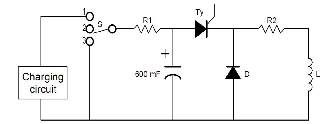
Typically, a diode (or another thyristor) and a resistor (the "crowbar resistor") are placed in parallel with the main circuit.

1. Pulse Rise: The capacitor discharges into the L-R series (the magnet). The diode blocks any current from flowing through the crowbar resistor.
2. Pulse Decay: After the peak, the voltage across the capacitor reverses. The crowbar diode becomes forward-biased, creating a new discharge path. The current now circulates in the local L-R loop formed by the magnet and the crowbar resistor, bypassing the capacitor.

The current decay is no longer sinusoidal. It becomes an exponential decay governed by the new L/R time constant of the crowbar loop: $I(t)\approx I_{peak}{e}^{-t/(L/R_{crowbar})}$. By choosing the crowbar resistance, a designer can precisely control the decay time, creating a much longer pulse tail than the natural RLC oscillation would allow.

The figure below from the arXiv paper LINK clearly illustrates the difference.

Figure 5 from 'Nuclear magnetic resonance spectroscopy in pulsed ...' (a) A simple LC circuit. (b) A more realistic pulsed-field circuit with a thyristor switch and a crowbar circuit. (c) The resulting current profiles. The black line is the fast oscillation of the simple LC circuit. The blue line shows the longer, shaped pulse achieved with the crowbar circuit.

Flat-Top and Controlled Waveforms

For ultimate control, facilities can generate even more complex pulse shapes. This often involves a second, smaller power supply connected to a compensation coil, which actively adds or subtracts field to hold the total field constant, creating a "flat-top" pulse.

The image below shows the variety of pulse shapes available at a major facility like the National High Magnetic Field Laboratory (NHMFL). You can see the standard capacitor-driven profiles (similar to our underdamped case) alongside highly engineered flat-top and linear ramp pulses.

Conclusion

In this lesson, we explored how the R, L, and C components of a pulsed magnet system govern the time evolution of the magnetic field. We moved beyond the low-loss approximation to understand the full spectrum of behaviors.

Key Takeaways:

• The pulse shape is determined by the damping ratio $\zeta =\frac{R}{2}\sqrt{C/L}$, which defines three regimes: underdamped (oscillatory), critically damped (fastest decay), and overdamped (slow decay).
• For a standard underdamped pulse, the duration is primarily set by the inductance and capacitance: $\tau \approx \pi \sqrt{LC}$. Increasing L or C creates a longer pulse.
• Pulse shapes can be modified. A crowbar circuit is commonly used to extend the pulse tail, changing the decay from sinusoidal to exponential with a time constant controlled by a crowbar resistor.
• The choice of L and C involves a critical trade-off. From our last lesson, $B_{peak}\propto 1/\sqrt{L}$. From this lesson, $\tau \propto \sqrt{L}$. Therefore, for a fixed capacitor bank energy, designing a coil for a longer pulse (higher L) will inherently result in a lower peak field.

Next Lesson Preview:

We have now established how to estimate a pulse's peak field and its duration. But how much does the coil heat up during one of these intense current pulses? The temperature rise is a critical factor that limits the magnet's performance and lifetime. In the next lesson, we will estimate the Joule heating and adiabatic temperature rise in a conductor during a single pulse, laying the groundwork for the thermal analysis of pulsed magnets.