Pulsed Magnet Figures of Merit

Introduction: Beyond a Single Number

It's tempting to think that the "best" magnet is simply the one that produces the highest field. While peak field is certainly a headline figure, it tells only part of the story. For an experimental physicist, other factors are often just as, or even more, important. Is the field uniform enough for a sensitive measurement? Is the pulse long enough for the sample to respond? Is there enough space to fit the cryostat?

A comprehensive evaluation requires a multi-faceted approach. We will now explore the four most important figures of merit that form the basis of pulsed magnet design and selection.

1. Peak Field ($B_{max}$)

The maximum magnetic field is the most prominent figure of merit. It's the primary driver for much of high-magnetic-field science, as higher fields can reveal new physical phenomena.

As we know from $B\propto I$, generating a higher field requires a larger peak current. This, in turn, demands more stored magnetic energy ($E_{mag}=\frac{1}{2}L{I}_{peak}^2$). However, simply pumping more energy into a coil is not a viable strategy. The achievable peak field is constrained by two fundamental physical limits:

1. Mechanical Limits: The Lorentz forces acting on the windings generate immense mechanical stress, particularly hoop stress, which scales with the square of the field ($\sigma \propto B^2$). At some point, this stress will exceed the ultimate tensile strength of the conductor and its reinforcement, leading to catastrophic failure.
2. Thermal Limits: The immense current density required for high fields leads to rapid Joule heating. In the adiabatic approximation, this causes a sharp temperature rise. The peak field is therefore also limited by the maximum temperature the conductor and its insulation can withstand before melting, annealing (softening), or breaking down.

As the text highlights, for non-destructive, long-pulse magnets (in the millisecond range), the primary challenge is surviving the immense electromagnetic forces. This mechanical limit is why fields in the ~60-100 T range represent the current frontier for this type of magnet.

2. Pulse Duration ($\tau$)

Pulse duration, often characterized by the rise time to peak field or the Full Width at Half Maximum (FWHM), is a critical parameter for the experimentalist.

The required duration is dictated by the physics of the experiment and the sample itself:

• Physical Phenomena: Some measurements, like nuclear magnetic resonance (NMR) or certain thermodynamic measurements, require the system to be in a "quasi-static" state, where the field changes slowly compared to the characteristic timescale of the phenomenon being studied.
• Eddy Currents: For conductive samples or metallic components in the sample holder (like a cryostat), a rapidly changing magnetic field will induce strong eddy currents. These currents can shield the sample from the applied field and cause significant heating, potentially destroying the sample or corrupting the measurement. A longer pulse provides time for the magnetic field to diffuse through these conductive materials.

The resource below gives a concrete example of this consideration.

Pulsed magnets can generate a wide variety of pulse shapes and durations, from microseconds to seconds. Capacitor-driven systems typically produce a half-sine waveform, while more complex power supplies can generate "flat-top" pulses where the field is held constant for a period.

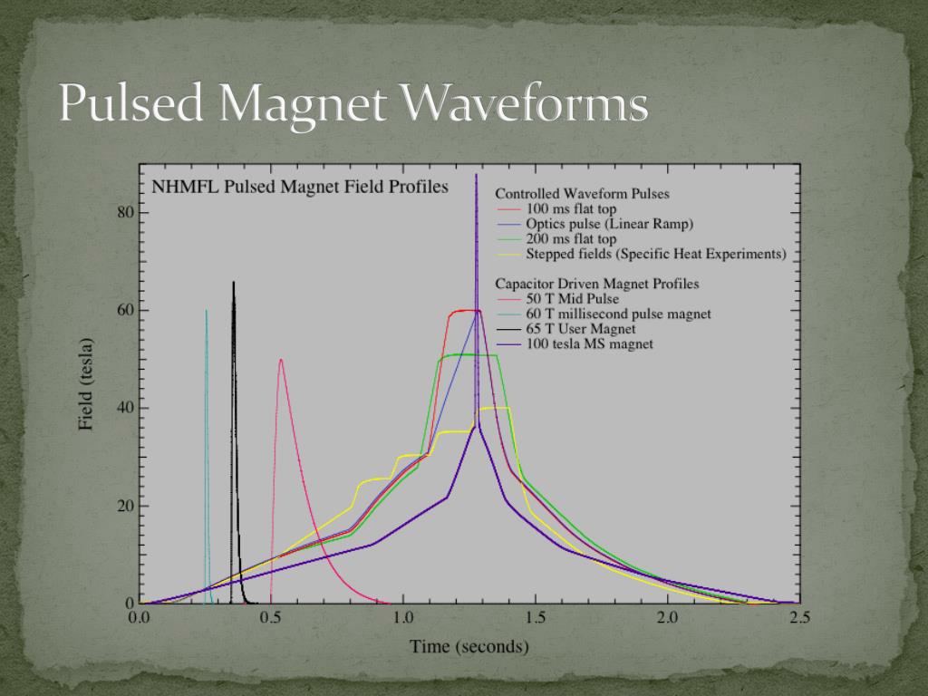
From our RLC circuit model, we know that the pulse rise time is approximately $t_{rise}\approx \frac{\pi }{2}\sqrt{LC}$. Therefore, achieving longer pulses requires increasing the coil's inductance ($L$) and/or the bank's capacitance ($C$), which generally leads to larger, more expensive, and more massive systems.

3. Field Homogeneity

Field homogeneity, or uniformity, measures the spatial variation of the magnetic field over the sample volume. It is typically expressed as the maximum field deviation relative to the central field ($\Delta B/B_0$) within a defined space, often a Diameter Spherical Volume (DSV).

For many experiments, high homogeneity is non-negotiable:

• NMR/EPR: These spectroscopic techniques rely on a precise relationship between frequency and magnetic field. Field gradients broaden the spectral lines, leading to a loss of resolution.
• Quantum Oscillations: Measurements like de Haas-van Alphen or Shubnikov-de Haas oscillations are sensitive to the field value. Inhomogeneity can "smear out" the oscillations.
• Phase Transitions: When studying sharp phase transitions, a non-uniform field means different parts of the sample will cross the transition at different times, blurring the measurement.

Field homogeneity is primarily a function of the coil's geometry. As a rule of thumb, a longer solenoid relative to its diameter (a higher aspect ratio) produces a more uniform field at its center.

Let's return to the Sandia paper to see how engineers quantify and verify homogeneity in a real-world design.

The paper reports impressive uniformity: within 1% for the MagLIF target and 1.7% for the MAPS configuration. This level of analysis is crucial to ensure the magnet will be suitable for its intended experiments.

4. Sample Volume (Bore Size)

The sample volume refers to the space available to the user at the center of the magnet, typically defined by the inner diameter of the coil, known as the bore.

The bore size is a critical practical parameter that dictates what can be measured in the magnet. A larger bore is needed to accommodate:

• Bulky sample environments like dilution refrigerators (for sub-Kelvin temperatures), diamond anvil cells (for high pressure), or complex optical setups.
• Larger samples, which can improve the signal-to-noise ratio in certain experiments.
• Extensive diagnostic access for probes, optical fibers, and wiring.

However, sample volume comes at a steep price. For a simple solenoid with a fixed amount of stored energy, the central field is inversely related to its dimensions. A larger bore inevitably means a lower peak field, all else being equal. This creates one of the most fundamental trade-offs in magnet design.

The design of the Sandia system again provides a clear illustration.

This is a perfect example of the trade-off in action: the 10 T design provides full diagnostic access. To reach a reliable 15 T, they must move to a "limited-access" configuration. To push towards 25-30 T, they must use a solid magnet with no radial diagnostic access at all. Each step up in field requires a sacrifice in access and, by extension, the types of experiments that can be performed.

Conclusion

We have now dissected the four primary figures of merit used to characterize pulsed magnets. It should be clear that designing a magnet is not about maximizing a single number, but about finding an optimal balance for a specific application.

Key Takeaways:

• Peak Field ($B_{max}$): The headline number, ultimately limited by the mechanical strength and thermal properties of the coil materials.
• Pulse Duration ($\tau$): A critical experimental parameter determined by circuit properties ($L,C$) and driven by the need to overcome eddy currents and match the timescales of the physics being studied.
• Field Homogeneity: A measure of spatial field uniformity, crucial for spectroscopic and precision measurements, and primarily determined by the coil's geometric aspect ratio.
• Sample Volume (Bore Size): The practical space available for the experiment, which is in direct and often harsh trade-off with the achievable peak field.

Next Lesson Preview:
In this lesson, we identified the key metrics and saw hints of the compromises between them. In our next lesson, we will formalize this by exploring the fundamental trade-offs between peak field, pulse duration, sample volume, and coil lifetime. We will see how these parameters are mathematically and physically interlinked, forcing designers to make difficult choices to achieve their goals.