VTI Temperature Control System Design

1. The Core Components: Sensing and Acting

Any control system relies on three fundamental actions: sensing the state of the system, acting to change that state, and a control logic to decide what action to take. Let's begin with the physical hardware for sensing and acting.

1.1. Sensing: Cryogenic Thermometry in High Fields

To control temperature, you must first measure it accurately. This is uniquely challenging in our application.

A good starting point for understanding the available sensor technologies is the following thesis, which provides a concise overview.

For cryogenic applications, Resistive Temperature Detectors (RTDs) are very common. Instead of platinum (Pt100/Pt1000) which loses sensitivity at low temperatures, specialized semiconductor composite resistors like Cernox™ or Rox™ are often used. They offer high sensitivity in the 1-300 K range.

However, all resistive sensors share a major vulnerability in our context: magnetoresistance. Their electrical resistance depends not only on temperature but also on the magnetic field. A 50 T pulse would render a standard temperature reading completely meaningless.

So, how is this problem solved in practice? The answer is meticulous calibration.

As the NIST paper demonstrates, the solution is to characterize the magnetoresistance of each thermometer for a specific magnetic field and temperature range. The control software then stores this calibration data (like the curves in Fig. 9) in a lookup table. During an experiment, the software reads the raw resistance, measures the magnetic field, and calculates the true temperature by correcting for the magnetoresistive effect. This is a perfect example of a multi-physics problem solved with software.

1.2. Acting: Heaters

The "muscle" of the temperature control system is the heater. In a VTI, temperature is stabilized by balancing a constant flow of cooling power (from liquid helium or nitrogen) with a precisely controlled amount of heating.

• Type: Heaters are typically simple resistive elements. Non-inductively wound wire or thin-film foil heaters laminated in an insulator like Kapton are common choices to minimize their interaction with the magnet's changing field.
• Placement: The placement of heaters and thermometers is a critical design choice that dictates the stability and accuracy of the system. They are often mounted together on a copper block, which acts as a thermal reservoir to provide uniform temperature. This assembly is then placed in good thermal contact with the sample mount.

The image below shows a real-world example of a sample probe, illustrating the integration of these components.

2. The Control Logic: From Simple PI to Advanced Strategy

With a sensor and an actuator, we now need the "brain" to connect them. This is the control logic, which is almost universally a Proportional-Integral-Derivative (PID) controller or a simplified variant.

2.1. PID Control Fundamentals

A PID controller calculates the difference (or "error", $E(t)$) between the desired temperature setpoint and the measured temperature. It then computes an output—the power to apply to the heater—based on three terms:

• Proportional (P): The output is proportional to the current error. A large error results in a large corrective action. This provides the primary response.
• Integral (I): The output is proportional to the accumulated error over time. This term drives the steady-state error to zero, correcting for small but persistent offsets.
• Derivative (D): The output is proportional to the rate of change of the error. This term anticipates future error and can dampen overshoot, leading to a faster settling time.

The total output is a weighted sum: $\text{Output}=K_{p}E(t)+K_i\int E(t)dt+K_d\frac{dE(t)}{dt}$.

For thermal systems, which have intrinsically slow dynamics, the derivative term (D) can be overly sensitive to sensor noise, leading to erratic heater output. Therefore, a Proportional-Integral (PI) controller is often sufficient and more robust.

2.2. Tuning a PI(D) Controller

The performance of the controller depends entirely on the gain values $K_p$, $K_i$, and $K_d$. The process of finding the optimal values is called tuning. There are systematic methods, like the Ziegler-Nichols method, that provide a good starting point based on the system's open-loop response (how it behaves without a controller).

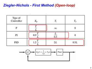
In practice, these initial values are almost always refined empirically ("by hand") to achieve the desired performance: fast response to setpoint changes with minimal overshoot and excellent stability against disturbances.

3. An Advanced System Architecture: The NIST Multi-Loop Design

A single PI loop driving a heater is a good start, but high-performance systems require a more sophisticated strategy to handle the large dynamic range of temperatures and heat loads. The NIST system provides an excellent case study of a state-of-the-art design.

The NIST design philosophy relies on a cascade of control loops:

1. Coarse Control (Loops #3 & #4): A pre-regulator intercepts the flow of cold helium gas coming from the main dewar. It has its own heater and thermometer (Loop #3). Its job is to pre-warm the gas to a temperature close to the final target temperature. The amount of gas flow is itself controlled by adjusting the pressure in the supply dewar (Loop #4). This is a crucial innovation: it buffers the sample from large fluctuations in the cooling power. Most of the heat generated by the high-current leads during a test is absorbed here, far from the sample.

2. Fine Control (Loops #1 & #2): Two separate heaters (H1 and H2) and thermometers (T1 and T2) are located at the top and bottom of the sample mount. These are the fine-tuning loops. They run at very low power (milliwatts) and are only responsible for making small, precise adjustments to bring the temperature of the pre-regulated gas to the exact setpoint.

This hierarchical or "cascade" design isolates the delicate task of fine temperature control from the "dirty" job of handling large, variable heat loads from the current leads and cryostat.

4. The Reality of Control: It's an Empirical Science

The final, and perhaps most important, lesson from the NIST paper is that even with this sophisticated design, achieving accurate temperature control is not a purely theoretical exercise. The system's behavior must be mapped empirically.

The key finding, as shown in their Figure 26, is that the heater power itself introduces a systematic error. Higher heater power creates larger thermal gradients between the heater, thermometer, and sample. This can cause the sample to be "sub-cooled" relative to what the thermometer reads.

This leads to a profound conclusion:

• To get the correct temperature, you must operate the heater at a specific power level.
• This "correct" heater power level is not constant; it depends on the other heat loads in the system (e.g., self-heating from the sample).
• Therefore, the control "logic" is not just a PID algorithm. It is a complete control protocol, empirically determined, where the software targets a specific heater power $H_2(I_{sample})$ as a function of the experimental conditions to minimize the temperature error.

This is the art and science of high-precision measurement: understanding and characterizing the limitations and subtle interactions of your own apparatus.

Conclusion

We have now designed a conceptual temperature control system for a VTI, moving from basic components to real-world complexities.

Key Takeaways:

• A VTI control system consists of thermometers (e.g., Cernox RTDs), heaters (e.g., resistive foils), and a control algorithm, typically PI logic.
• The primary challenge for thermometry in high fields is magnetoresistance, which must be corrected for using detailed, field-dependent calibration tables.
• High-performance systems employ a multi-loop or cascade strategy, using a pre-regulator for coarse control to buffer the fine control loop near the sample from large heat loads.
• Achieving millikelvin accuracy requires an empirically derived control protocol, not just a simple PID loop. The controller must actively manage thermal gradients by targeting specific heater power levels that are known to minimize measurement error under given conditions.

Next Lesson Preview

Having designed the thermal environment, we are now ready to place an experiment inside it. In our next lesson, we will tackle the challenge of performing sensitive electrical measurements in this noisy environment. We will design a system for resistivity or Hall effect measurements, addressing challenges like large inductive voltage pickup. This will take us into the heart of data acquisition in pulsed magnetic fields.