Resistivity & Hall Effect Measurements: Overcoming Inductive Challenges

1. The Measurement and the Overwhelming Challenge

First, let's briefly revisit the standard techniques before introducing the complication of the pulsed field.

• Resistivity: Typically measured using a four-probe (or van der Pauw) configuration. A known current $I$ is passed through two outer contacts, and the resulting voltage $V$ is measured across two inner contacts. The resistance is $R=V/I$, from which resistivity $\rho$ is calculated based on the sample's geometry.
• Hall Effect: This requires a transverse measurement. With current $I$ flowing along the sample and a magnetic field $B$ applied perpendicularly, a Hall voltage $V_H$ develops across the sample, perpendicular to both $I$ and $B$. This voltage is proportional to the field and inversely proportional to the charge carrier density.

In both cases, the voltage signal from the sample ($V_{\text{sample}}$) is often very small, typically in the microvolt (µV) to millivolt (mV) range.

1.1 The Problem: Inductive Voltage Pickup

Now, let's place our experiment inside a pulsed magnet. According to Faraday's Law of Induction, any closed loop of wire with area $A$ subjected to a time-varying magnetic flux ${\Phi }_B$ will have an electromotive force (EMF) or voltage induced in it:

The wiring for our voltage measurement—the two leads running from the sample to our measurement device—inevitably forms such a loop. In a pulsed magnet, the rate of change of the magnetic field, $dB/dt$, is enormous. For a typical 60 T, 100 ms pulse, the average $dB/dt$ can be over 1000 T/s.

To understand the scale of this problem, we can perform a simple calculation. The following resource provides an excellent, concise derivation.

Let's adapt their result for our scenario. If the voltage leads form a loop of area $A$ perpendicular to the field, the induced voltage is simply $V_{\text{pickup}}=-A\frac{dB}{dt}$.

Consider a very small, well-designed loop with an area of just 1 mm² ($10^{-6}$ m²). With a $dB/dt$ of 1000 T/s:
$V_{\text{pickup}}=(10^{-6}{\text{ m}}^2)\times (1000\text{ T/s})=1\text{ mV}$
Even this optimistic case gives a pickup voltage of 1 mV. In reality, with connectors and imperfect wiring, the loop area is often larger, leading to pickup voltages of 10s or even 100s of mV.

The core challenge is clear: we need to measure a µV-level signal from our sample in the presence of a mV-level (or larger) noise signal that is 1,000 to 100,000 times stronger.

2. First Line of Defense: Probe and Wiring Design

Our first goal is to minimize the induced voltage at its source by carefully designing the physical wiring. The principle is simple: minimize the effective loop area $A$ of the voltage measurement circuit.

The 'Inductive Cross-Talk' note you just read outlines several practical strategies to achieve this.

The most effective and common technique is to use a twisted pair for the voltage leads. By twisting the 'V+' and 'V-' wires together, you create a series of small loops with alternating orientation to the magnetic field. The induced voltage in one loop is nearly cancelled by the opposing voltage in the next, drastically reducing the net loop area and thus the total pickup voltage. For even better performance, miniature coaxial cables can be used, where the shield serves as one conductor and the central wire as the other, providing excellent screening.

The image below, from a thesis developed at LNCMI, shows the intricate assembly of a probe head designed for pulsed fields. While it's for optical spectroscopy, the principles of miniaturization and dense component packing are the same. Every wire's path must be meticulously planned to minimize loop areas.

3. Second Line of Defense: AC Measurement and Lock-in Detection

While good wiring is essential, it can never perfectly eliminate the inductive pickup. The next layer of our defense is to use signal processing to distinguish the desired signal from the noise. This is where your experience with lock-in amplifiers becomes central.

The strategy involves a fundamental shift in the measurement:

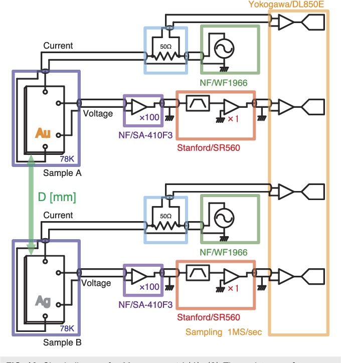
1. Excite with AC: Instead of a DC current, we drive the sample with a high-frequency AC current, typically between 10 kHz and 100 kHz. The voltage across the sample is now also an AC signal at the same high frequency.
2. Frequency Separation: We now have two signals mixed together:
   • Our Signal: A small AC voltage at a high frequency $f_{\text{signal}}$ (e.g., 50 kHz).
   • The Noise: A large induced voltage whose time profile follows the magnet pulse, which is a very low-frequency event (a single rise and fall over ~100 ms, corresponding to frequencies of ~10 Hz).
3. Detect with a Lock-in: A lock-in amplifier is precisely the tool needed to separate these. It acts as an extremely narrow band-pass filter centered exactly at the signal frequency, rejecting the massive, low-frequency inductive pulse.

To refresh our understanding of how a lock-in achieves this, let's watch a short video.

The concept of Dynamic Reserve is crucial. A dynamic reserve of 120 dB, as mentioned in the video, means the instrument can accurately measure a signal even in the presence of noise that is $10^{120/20}=10^6$ times larger. This is what allows a lock-in to recover a 1 µV signal floating on top of a 1 V inductive background.

The complete measurement chain would look like this:

4. Advanced Technique: Active Compensation

In extreme cases, the inductive pickup can be so large that it saturates the input of the very first electronic component in the chain—the preamplifier. If the preamp is saturated (or "railed"), the signal is clipped and irretrievably lost before it even reaches the lock-in amplifier.

To solve this, we can implement an active compensation scheme.

• Principle: We deliberately create a second, small "compensation coil" and place it near the sample's voltage wiring loop.
• Implementation: This coil is just a few turns of fine wire. It will also experience an inductive pickup $V_{\text{comp}}\approx -A_{\text{comp}}\frac{dB}{dt}$.
• Subtraction: This compensation voltage is then subtracted from the raw signal from the sample's voltage leads, before the preamplifier.
  $V_{\text{input to preamp}}=(V_{\text{sample}}+V_{\text{pickup}})-V_{\text{comp}}$
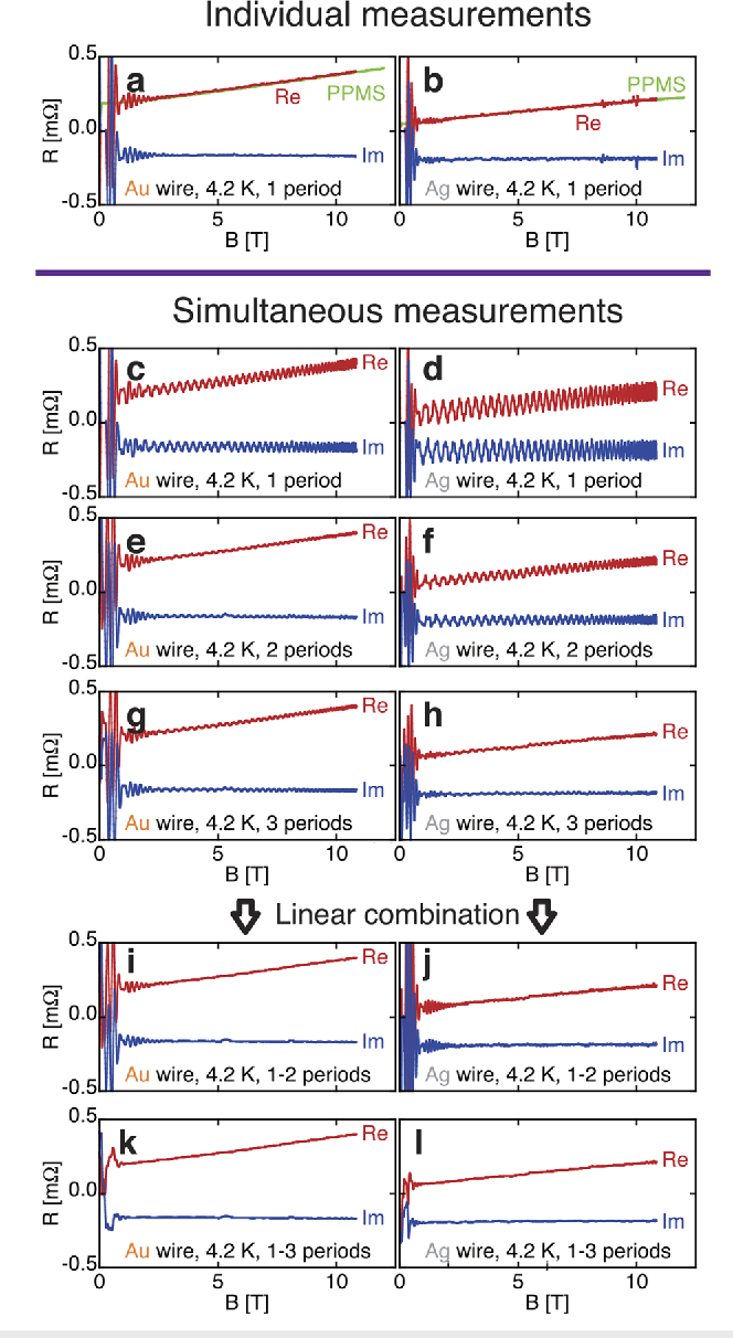
  By carefully adjusting the area and orientation of the compensation coil (often by routing its signal through a potentiometer to fine-tune the subtraction factor), one can make $V_{\text{comp}}$ almost exactly equal to $V_{\text{pickup}}$. The massive pickup is cancelled out, leaving only the small $V_{\text{sample}}$ to be amplified and measured by the lock-in.

The image below shows real data from a pulsed-field experiment. The imaginary part of the resistance, Im(R), is directly proportional to the uncompensated inductive signal. The goal of active compensation is to make this component as close to zero as possible.

Conclusion

We have designed a robust system for electrical transport measurements in the extreme environment of a pulsed magnet. Success relies not on a single magic bullet, but on a layered defense strategy.

Key Takeaways:

• The Challenge: The large $dB/dt$ in a pulsed magnet induces a voltage in measurement leads that can be orders of magnitude larger than the physical signal from the sample.
• Layer 1 (Hardware): Meticulous probe design and wiring, primarily using twisted pairs or coaxial cables for voltage leads, is the first and most critical step to minimize the inductive loop area.
• Layer 2 (Electronics/Signal Processing): Using an AC current excitation and a lock-in amplifier allows for the separation of the high-frequency sample signal from the low-frequency inductive background. The dynamic reserve of the lock-in is the key performance parameter.
• Layer 3 (Advanced Hardware): For extreme cases where the pickup threatens to saturate the preamplifier, an active compensation circuit using a secondary pickup coil can be used to subtract the inductive voltage before amplification.

Next Lesson Preview

In this lesson, we treated inductive pickup as a nuisance to be eliminated. In our next lesson, we will embrace it. We will learn how to design a magnetization measurement system where the signal of interest is the voltage induced by the sample's changing magnetic moment. We will design a magnetization measurement system using compensated pickup coils suitable for pulsed fields, turning our enemy into our measurement tool.