Graphing Linear Equations: Slope-Intercept Form

Welcome back! In our last lesson, we mastered plotting individual points on the Cartesian plane, giving a "visual home" to pairs of numbers. You learned how an ordered pair (x, y) corresponds to a unique address on a grid.

Today, we'll discover that when the points come from a specific type of function—a linear function—they don't scatter randomly. Instead, they line up perfectly. We will learn to graph the equation of a line, $y = m x + b$ , by understanding its two key components: the slope (m) and the y-intercept (b). This skill is fundamental because it transforms an abstract algebraic equation into a concrete geometric object, a line, which is one of the foundational elements of linear algebra.

The Anatomy of a Line: Slope-Intercept Form

Any straight line on a 2D plane can be described by a wonderfully simple equation called the slope-intercept form:

y = m x + b

This equation is like a recipe for a line. It tells you exactly how to draw it.

x and y are the coordinates of any point on the line. They are the variables that link the horizontal and vertical positions.
m and b are the line's defining characteristics. Once you know them, you know everything about the line.

Let's break down what m and b mean.

This image provides a great overview of the slope-intercept form. It defines each component and shows how `m` (slope) and `b` (y-intercept) relate to the line's graph.

As you can see, b tells us where the line starts on the y-axis, and m tells us how steep it is. Let's investigate each of these parameters more closely.

The Y-Intercept (`b`): Your Starting Point

The easiest part of a line to find is often its y-intercept. This is the point where the line crosses the vertical y-axis.

Think about any point on the y-axis. What do all those points have in common? Their x-coordinate is always 0. So, if we plug $x = 0$ into our equation:

y = m (0) + b

y = 0 + b

y = b

This tells us that the line crosses the y-axis at the point (0, b). The value b in the equation gives you the y-coordinate of your starting point. It anchors the line in place.

Let's watch a segment of a video that visualizes this concept perfectly.

Basic Linear Functions - Math Antics

This video from Math Antics provides an excellent intuitive explanation for how the 'b' value works.

Please watch the portion from the introduction of 'b' to where the term "y-intercept" is defined. Notice how changing the value of b simply shifts the entire line up or down without changing its steepness.

The Slope (`m`): The Direction and Steepness

If the y-intercept is the line's starting point, the slope tells you where to go from there. The slope, m, describes both the direction and the steepness of the line. It's defined as the "rise over run".

Rise over Run: This is the ratio of the vertical change (rise) to the horizontal change (run) between any two points on the line.

m = \frac{change in y}{change in x} = \frac{rise}{run}

This means for every 1 unit you move to the right along the x-axis, the line goes up or down by m units.

Positive Slope (m > 0): The line goes uphill from left to right. A larger m means a steeper climb.
Negative Slope (m < 0): The line goes downhill from left to right.
Zero Slope (m = 0): The line is perfectly horizontal. The "rise" is zero.

The next video segment will give you a strong intuition for how the value of m affects the line's graph.

Basic Linear Functions - Math Antics

We'll return to the Math Antics video to see how the slope 'm' works.

Watch from the introduction of y=mx. Pay close attention to how different values of m—positive, negative, fractional, and zero—change the steepness and direction of the line.

To formalize this, the slope between two points $(x_{1}, y_{1})$ and $(x_{2}, y_{2})$ is calculated with the formula:

m = \frac{y _{2} - y _{1}}{x _{2} - x _{1}}

Let's see a quick demonstration of this calculation.

Graphing Lines in Algebra: Understanding Slopes and Y-Intercepts

This clip from Professor Dave Explains clearly shows how to apply the "rise over run" formula.

Watch the segment from where the slope is calculated. This connects the visual idea of rise/run to the mathematical formula.

How to Graph a Line Using `y = mx + b`

Now we can combine these two pieces of information into a simple, two-step process to graph any linear equation.

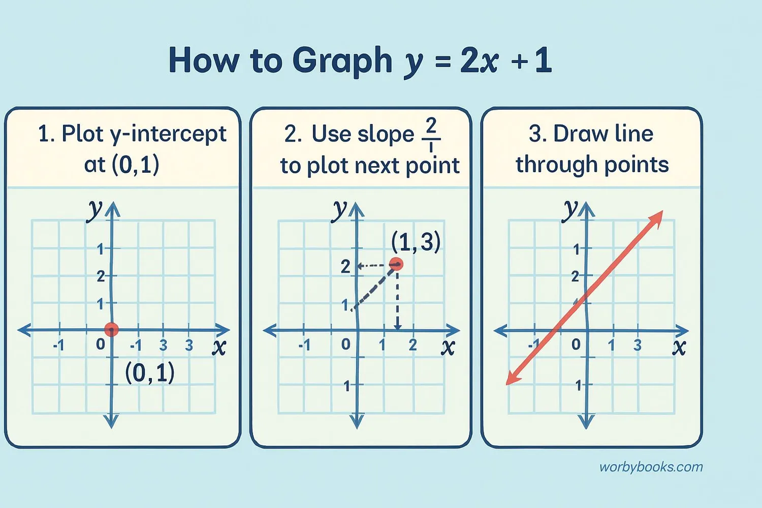
Let's use the example equation $y = 2 x + 1$ .

Plot the y-intercept (b).
First, identify b. In $y = 2 x + 1$ , b = 1. So, our starting point is at (0, 1). Go to the origin, and move 1 unit up on the y-axis. Plot that point.
Use the slope (m) to find a second point.
Next, identify m. In $y = 2 x + 1$ , m = 2. It's helpful to think of any whole number slope as a fraction: $m = \frac{2}{1}$ . This means "rise 2, run 1".
Starting from your y-intercept (0, 1), rise 2 units (go up 2) and then run 1 unit (go right 1). Plot this new point at (1, 3).
Draw the line.
With two points plotted, you can now use a ruler or straight edge to draw a line that passes through both of them. This line represents all possible solutions to the equation $y = 2 x + 1$ .

This exact process is illustrated perfectly in the following image.

This image shows the three simple steps to graph a line: 1. Plot the y-intercept. 2. Use the slope (rise/run) to find a second point. 3. Draw a line through the two points.

This method is powerful because it works for any linear equation. Let's review a textual guide that reinforces these steps.

Slope Intercept Form of Linear Equations: A Guide - Statistics By Jim

This article from "Statistics By Jim" clearly explains the components and provides a step-by-step guide for graphing.

First, read the section Interpreting the Coefficients to solidify your understanding of m and b. Then, read the next section, How to Graph, which summarizes the method we just discussed.

Explore for Yourself

To build a really strong intuition, there's no substitute for experimentation. The following link takes you to an interactive graph where you can change the slope and intercept with sliders and see the line change in real time.

Interactive Graph: Intercept and Slope

This interactive tool by Elena Llaudet lets you directly manipulate 'm' and 'b' to see their effect on the graph.

Read the introductory text defining the intercept and slope. Then, use the sliders at the bottom of the page to change the values for the intercept and slope. Move the intercept slider: Watch how the line moves up and down, but its angle stays the same. Move the slope slider: See how the line pivots around the y-intercept, getting steeper or flatter. Try making the slope positive, negative, and zero.

Conclusion

Today, we've unlocked the connection between an algebraic equation and its geometric picture. By understanding the slope-intercept form, $y = m x + b$ , you can now look at an equation and immediately visualize the line it represents.

Here are the key takeaways:

The equation $y = m x + b$ is the slope-intercept form for a straight line.
The y-intercept (b) is the point where the line crosses the y-axis, giving us a starting coordinate of (0, b).
The slope (m) is the "rise over run," telling us the line's steepness and direction.
To graph a line, you can use a simple two-step process: plot the y-intercept, then use the slope to find a second point.

In our next lesson, we will build directly on this skill. Now that we can graph and interpret a single line, we'll ask: what happens when two lines exist on the same plane? They might intersect, run parallel to each other, or lie on top of one another. Exploring this question will lead us directly into the concept of systems of linear equations, a cornerstone of linear algebra.

Recommended resources

The Anatomy of a Line: Slope-Intercept Form

The Y-Intercept (b): Your Starting Point

The Slope (m): The Direction and Steepness

How to Graph a Line Using y = mx + b

Explore for Yourself

Conclusion

The Y-Intercept (`b`): Your Starting Point

The Slope (`m`): The Direction and Steepness

How to Graph a Line Using `y = mx + b`