Disjunctive Graphs for Job Shop Problems

Why Do We Need a Special Graph?

The challenge of the JSSP lies in the dual nature of its constraints:

1. Precedence Constraints: Operations within a single job must follow a strict sequence (e.g., drilling must happen before painting).
2. Resource Constraints: A machine can only process one operation at a time. If two different jobs need the same machine, one must wait for the other.

A disjunctive graph is a model that elegantly captures both types of constraints simultaneously. It provides a complete representation of the entire problem, not just a single potential schedule.

Anatomy of a Disjunctive Graph

The best way to understand the disjunctive graph is by studying its components. We'll use a formal definition and then break it down with a practical example.

Based on your reading, let's summarize the key components of a disjunctive graph $G=(V,C\cup D)$:

• Nodes (V):

  • Each operation of each job is represented by a node.
  • We add two special, fictitious nodes: a source node s (or 0) representing the start of the schedule, and a sink node t (or *) representing the end.
  • Each operation node has a "weight" equal to its processing time. The source and sink nodes have a weight of 0.

• Conjunctive Arcs (C):

  • These are directed arcs (solid lines) that connect consecutive operations of the same job.
  • They represent the fixed technological routing or precedence constraints. For example, if Job 1 requires OpA then OpB, we add a directed arc OpA -> OpB.
  • These are called "conjunctive" because all of these precedence relations must be respected in any valid schedule.

• Disjunctive Arcs (D):

  • These are pairs of directed arcs (often drawn as a single dashed or colored line for simplicity) that connect all operations that must be processed on the same machine.
  • For any two operations i and j that need the same machine, we have a disjunction: either i is processed before j (represented by arc i -> j), or j is processed before i (represented by arc j -> i).
  • These are "disjunctive" because for each pair, we must choose one of the two possible orderings to create a valid schedule.

Constructing a Disjunctive Graph: A Step-by-Step Example

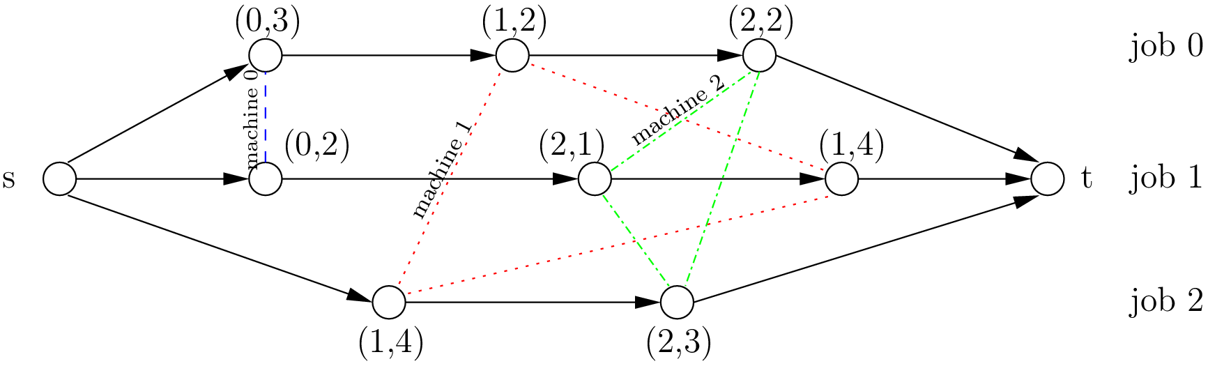
Let's solidify this by building a disjunctive graph for the 3-job, 3-machine problem described in the reading material.

Problem Data:

• Job 0: (M0, p=3) -> (M1, p=2) -> (M2, p=2)
• Job 1: (M0, p=2) -> (M2, p=1) -> (M1, p=4)
• Job 2: (M1, p=4) -> (M2, p=3)

Let's denote the k-th operation of job j as $O_{jk}$.

Step 1: Create Nodes
Create a node for each operation, plus the source (s) and sink (t).

• Job 0: $O_{00}$, $O_{01}$, $O_{02}$
• Job 1: $O_{10}$, $O_{11}$, $O_{12}$
• Job 2: $O_{20}$, $O_{21}$

Step 2: Add Conjunctive Arcs
Connect the operations for each job in their specified sequence. Also, connect the source s to the first operation of each job, and the last operation of each job to the sink t.

• Job 0: s -> O_00 -> O_01 -> O_02 -> t
• Job 1: s -> O_10 -> O_11 -> O_12 -> t
• Job 2: s -> O_20 -> O_21 -> t

Step 3: Add Disjunctive Arcs
Connect all operations that share a machine.

• Machine 0: $O_{00}$ and $O_{10}$ are connected.
• Machine 1: $O_{01}$, $O_{12}$, and $O_{20}$ are all connected to each other, forming a "clique" of 3 operations.
• Machine 2: $O_{02}$, $O_{11}$, and $O_{21}$ form another clique.

The resulting graph should look exactly like the one in the resource you reviewed.

Interpreting the Graph: From Problem to Solution

The disjunctive graph represents the problem. So, how does it represent a solution?

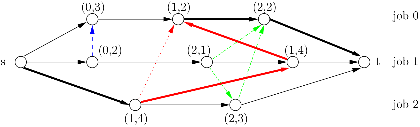
A solution to the JSSP is found by making a decision for every disjunctive arc. For each pair of operations on the same machine, you must choose their processing order. This is equivalent to selecting one direction for each disjunctive arc.

For example, on Machine 0, you must decide whether to schedule Job 0 before Job 1 (O_00 -> O_10) or Job 1 before Job 0 (O_10 -> O_00). When you have made a choice for every pair on every machine, you have a complete schedule.

A feasible schedule corresponds to a selection of disjunctive arcs that results in a Directed Acyclic Graph (DAG). If your choices create a cycle (e.g., A -> B on a machine, but B's successor must precede A's predecessor), the schedule is impossible.

Once you have a feasible schedule (a DAG), you can determine the makespan ($C_{max}$). The makespan is simply the length of the longest path from the source s to the sink t. This path is called the critical path, as any delay to an operation on this path will delay the entire schedule.

The length of a path is calculated by summing the processing times (node weights) of all operations along that path.

The image below shows the same graph after all disjunctive choices have been made. The disjunctive arcs are now directed, and the critical path, which determines the makespan, is highlighted.

Conclusion

In this lesson, you have learned how to model a Job Shop Scheduling Problem using a disjunctive graph. This powerful representation is a cornerstone of scheduling research because it captures the problem's inherent structure—the interplay between precedence and resource constraints.

Key Takeaways:

• A disjunctive graph models a JSSP with nodes for operations, conjunctive arcs for job precedence, and disjunctive arcs for machine resource conflicts.
• Constructing the graph involves creating nodes for operations, adding directed conjunctive arcs for job routes, and adding undirected disjunctive arcs for shared machines.
• Solving the JSSP is equivalent to converting the disjunctive graph into a directed acyclic graph (DAG) by choosing a direction for each disjunctive arc.
• The makespan ($C_{max}$) of a given schedule is the length of the longest path (critical path) from source to sink in the corresponding DAG.

Preview of the Next Lesson:

Now that we can represent a schedule and calculate its makespan using the graph, the next logical step is to formalize this calculation. In the next lesson, you will learn how to calculate the makespan as the longest path in a disjunctive graph. We will explore the critical path method algorithm, which is an efficient way to find this longest path and determine the earliest start times for all operations in a fixed schedule. This is a crucial building block for nearly all advanced scheduling algorithms.