Makespan as Longest Path in Disjunctive Graphs

The General Problem: Longest Path in a DAG

Before we tackle the disjunctive graph specifically, let's look at the underlying computer science problem: finding the longest path in any Directed Acyclic Graph (DAG). The structure of this problem and its solution should be familiar given your background in analysis.

A key property of a DAG is that it can be topologically sorted, meaning we can order its vertices so that for every directed edge from vertex u to v, u comes before v in the ordering. This property is what allows for an efficient algorithm.

Adapting the Algorithm for Scheduling

The video provides the core logic, but we need to make one important adaptation for our scheduling context. In the video's example, each node (a course) represents one unit of time (a semester). In our disjunctive graph, each node (an operation) has its own specific duration, its processing time $p_{ij}$.

Therefore, the "length" of a path is not the number of nodes, but the sum of the processing times of the nodes on that path.

The longest path from the source s to an operation node (i,j) has a crucial physical interpretation: it is the earliest possible start time for that operation in the given schedule. Let's call this ES_{ij}.

The algorithm to find the makespan is a formal procedure for calculating these earliest start times for all operations, culminating in the completion of the final operation.

The Critical Path Algorithm

As the reading describes, we can calculate the earliest start time for every operation by moving forward through the graph. An operation can only begin after all its preceding operations (both from the same job and on the same machine) are finished.

Let's formalize the algorithm:

1. Initialization:
   • The source node s represents the start of time. Its earliest start time is ES_s = 0. Its "completion time" is also 0 since it has no duration.
2. Forward Pass:
   • For any operation node (i,j), its earliest start time ES_{ij} is the maximum of the completion times of all its immediate predecessors in the DAG.
   • Let Pred(i,j) be the set of immediate predecessors of node (i,j). The completion time of a predecessor (k,l) is ES_{kl} + p_{kl}.
   • The formula is: $$E{S}_{ij}=\underset{(k,l)\in Pred(i,j)}{\max }\{E{S}_{kl}+p_{kl}\}$$
   • You repeat this calculation for all nodes, following the topological sort of the graph (which is naturally enforced by the dependencies).
3. Makespan Calculation:
   • The sink node t can only "start" when all operations preceding it are complete. The makespan C_{max} is therefore the earliest start time of the sink node t. $$C_{max}=E{S}_t=\underset{\text{all final ops }(i,j)}{\max }\{E{S}_{ij}+p_{ij}\}$$

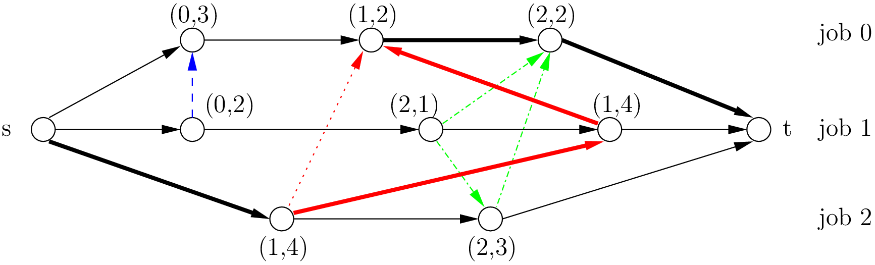
The sequence of nodes and arcs that determines the final C_{max} value is called the critical path. Any delay to an operation on this path will directly increase the makespan.

A Worked Example

Let's apply this algorithm to the 2-job, 2-machine problem from the last lesson's quiz.

• Job 1: $O_{11}$(M1, p=5) -> $O_{12}$(M2, p=3)
• Job 2: $O_{21}$(M2, p=2) -> $O_{22}$(M1, p=4)

Let's assume we have chosen a schedule where on M1, Job 1 runs before Job 2, and on M2, Job 2 runs before Job 1.

• M1 sequence: $O_{11}\to O_{22}$
• M2 sequence: $O_{21}\to O_{12}$

The predecessors for each node are:

• Pred(O_11) = {s}
• Pred(O_21) = {s}
• Pred(O_12) = {O_11 (job), O_21 (machine)}
• Pred(O_22) = {O_21 (job), O_11 (machine)}
• Pred(t) = {O_12, O_22}

Now, let's calculate:

1. ES_s = 0
2. ES_{11} = ES_s + p_s = 0. Completion time C_{11} = 0 + 5 = 5.
3. ES_{21} = ES_s + p_s = 0. Completion time C_{21} = 0 + 2 = 2.
4. ES_{12} = max(C_{11}, C_{21}) = max(5, 2) = 5. Completion time C_{12} = 5 + 3 = 8.
5. ES_{22} = max(C_{21}, C_{11}) = max(2, 5) = 5. Completion time C_{22} = 5 + 4 = 9.
6. C_{max} = ES_t = max(C_{12}, C_{22}) = max(8, 9) = 9.

The makespan for this schedule is 9. The critical path is s -> O_11 -> O_22 -> t.

Conclusion

In this lesson, we have connected the graphical representation of a schedule to a quantitative performance measure, the makespan. By understanding that makespan is equivalent to the longest path in a DAG, we can use a straightforward and efficient algorithm to calculate it.

Key Takeaways:

• For any feasible schedule (a DAG), the makespan ($C_{max}$) is the length of the longest path from the source to the sink, also known as the critical path.
• The length of a path is the sum of the processing times of the operation nodes on it.
• The length of the longest path to a node (i,j) represents the earliest start time (ES_{ij}) for that operation.
• The algorithm computes these earliest start times in a forward pass, using the formula: $E{S}_{ij}={\max }_{(k,l)\in Pred(i,j)}\{E{S}_{kl}+p_{kl}\}$.
• The makespan is the maximum completion time over all final operations: $C_{max}={\max }_{\text{all final ops}}\{E{S}_{ij}+p_{ij}\}$.

Preview of the Next Lesson:

We have now learned how to construct a graph for a JSSP and how to evaluate a given schedule from that graph. However, we have been assuming that a schedule (a selection of disjunctive arcs) is given to us. The next logical question is: how do we generate good schedules in the first place?

In our next lesson, we will begin to answer this by learning about the Giffler-Thompson algorithm, a classic method for constructing active schedules. An active schedule is one in which no operation can be started earlier without delaying another. This set of schedules is important because it is guaranteed to contain at least one optimal solution, allowing us to narrow our search.