Giffler-Thompson Algorithm for Job Shop Scheduling

Why Active Schedules?

Before we dive into the algorithm itself, we need to understand its goal: to generate active schedules. The search for an optimal schedule can be narrowed down considerably if we focus on specific classes of schedules.

As the reading highlights, there are three key types of feasible schedules:

• Semi-active: No operation can be started earlier without changing the sequence of operations on some machine. This is a very basic notion of a "compact" schedule.
• Active: No operation can be started earlier without either delaying another operation or violating its job's precedence constraints.
• Non-delay: No machine is kept idle if there is an operation waiting to be processed on it.

The relationship between these sets is: Non-delay ⊂ Active ⊂ Semi-active.

The most important takeaway, as stated in the paper, is that for minimizing makespan (and other regular objectives), an optimal schedule is always an active schedule. This powerful result means we don't have to search the entire space of all possible schedules; we can restrict our search to the set of active schedules, which is significantly smaller yet guaranteed to contain the optimum. This is precisely what the Giffler-Thompson algorithm helps us do.

The Giffler-Thompson Algorithm

The Giffler-Thompson (GT) algorithm, developed in 1963, is an iterative procedure that constructs an active schedule by making one scheduling decision at a time. At each step, it identifies a point of conflict and resolves it.

Let's study the formal steps of the algorithm.

Let's break down the logic of the algorithm using the notation from the paper:

1. Initialization (Step 1):

   • You start with an empty partial schedule $P_1$.
   • The set of "schedulable" operations, $S_1$, contains the first operation of every job, as none of them have predecessors.

2. Iterative Scheduling (Steps 2-5): This is a loop that continues until all operations are scheduled. In each iteration t:

   • Identify the next critical event (Step 2): For every operation $o_k$ in the current set of schedulable operations $S_t$, calculate its earliest possible start time ${\rho }_k$ and its earliest possible completion time $b_k={\rho }_k+p_k$. The earliest start time ${\rho }_k$ is determined by the completion time of its immediate job predecessor (if any) and the time the required machine becomes free. We then find the operation that could finish the earliest, and call its completion time $b^{\ast }$ and its machine $M^{\ast }$. This represents the next moment a machine will complete a critical task.
   • Form the Conflict Set (Step 3): This is the core of the algorithm. We create a set of all operations in $S_t$ that require machine $M^{\ast }$ and could start before the critical event time $b^{\ast }$. This is the set of operations that are in conflict for machine $M^{\ast }$.
   • Make a Decision (Implicit in Step 3): The algorithm states to "Choose an operation $o_j$" from this conflict set. This is the decision point. The GT algorithm itself is a framework; to implement it as a heuristic, you must use a priority rule (e.g., Shortest Processing Time, First-In-First-Out, or even randomly) to select which operation from the conflict set to schedule. If you were to explore all possible choices at each step, you would generate the entire set of active schedules.
   • Update and Continue (Step 4 & 5): The chosen operation $o_j$ is added to the schedule. It is removed from $S_t$, and its direct successor (from the same job, if one exists) is added to the set of schedulable operations, creating $S_{t+1}$. The loop then repeats.

A Worked Example

Let's apply the GT algorithm to the following 3-job, 3-machine problem.

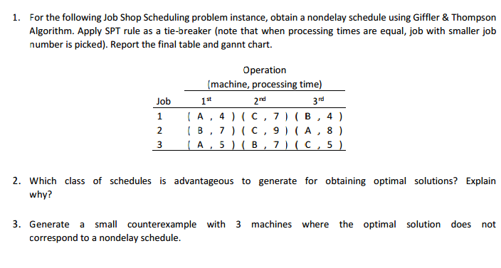
The operations are:

• Job 1: $O_{11}$(M1, 3), $O_{12}$(M2, 2), $O_{13}$(M3, 2)
• Job 2: $O_{21}$(M2, 2), $O_{22}$(M1, 4), $O_{23}$(M3, 1)
• Job 3: $O_{31}$(M3, 4), $O_{32}$(M2, 1), $O_{33}$(M1, 3)

Let's trace the first few iterations. We will use the Shortest Processing Time (SPT) rule to make decisions when conflicts arise.

Iteration 1 (t=1):

• Schedulable Set $S_1$: { $O_{11}$, $O_{21}$, $O_{31}$ }
• Earliest Times:
  • $O_{11}$: ${\rho }_{11}=0$, $b_{11}=0+3=3$ on M1
  • $O_{21}$: ${\rho }_{21}=0$, $b_{21}=0+2=2$ on M2
  • $O_{31}$: ${\rho }_{31}=0$, $b_{31}=0+4=4$ on M3
• Critical Event (Step 2): $b^{\ast }=\min (3,2,4)=2$, which belongs to $O_{21}$ on machine $M^{\ast }=$ M2.
• Conflict Set (Step 3): We need operations in $S_1$ that require M2 and can start before $b^{\ast }=2$. Only $O_{21}$ uses M2, and its start time ${\rho }_{21}=0<2$. So, the conflict set is { $O_{21}$ }.
• Decision: There is only one choice. We schedule $O_{21}$. Completion time $C_{21}=2$.
• Update (Step 4): $S_2$ = { $O_{11}$, $O_{31}$, $O_{22}$ } (where $O_{22}$ is the successor of $O_{21}$).

Iteration 2 (t=2):

• Schedulable Set $S_2$: { $O_{11}$, $O_{31}$, $O_{22}$ }
• Earliest Times:
  • $O_{11}$ (M1): ${\rho }_{11}=0$, $b_{11}=0+3=3$
  • $O_{31}$ (M3): ${\rho }_{31}=0$, $b_{31}=0+4=4$
  • $O_{22}$ (M1): Its predecessor $O_{21}$ finishes at time 2. So, ${\rho }_{22}=2$, $b_{22}=2+4=6$.
• Critical Event (Step 2): $b^{\ast }=\min (3,4,6)=3$, belonging to $O_{11}$ on machine $M^{\ast }=$ M1.
• Conflict Set (Step 3): Operations in $S_2$ using M1 with $\rho <3$.
  • $O_{11}$: uses M1, ${\rho }_{11}=0<3$. Yes.
  • $O_{22}$: uses M1, ${\rho }_{22}=2<3$. Yes.
  • $O_{31}$: uses M3. No.
  • The conflict set is { $O_{11}$, $O_{22}$ }.
• Decision: Now we have a choice. We apply our SPT rule.
  • Processing time of $O_{11}$ is 3.
  • Processing time of $O_{22}$ is 4.
  • SPT selects $O_{11}$. We schedule $O_{11}$. Completion time $C_{11}=3$.
• Update (Step 4): $S_3$ = { $O_{31}$, $O_{22}$, $O_{12}$ }.

The Non-Delay Variant

The GT algorithm can be slightly modified to produce non-delay schedules. As we know, this is a more restrictive subset of active schedules.

The modification, described in resource LINK, changes Step 2 and 3: instead of finding the minimum completion time $b^{\ast }$, you find the minimum start time ${\rho }^{\ast }$. You then choose from the operations that can start at that earliest time on the corresponding machine. This ensures no machine is ever left idle if an operation is available for it.

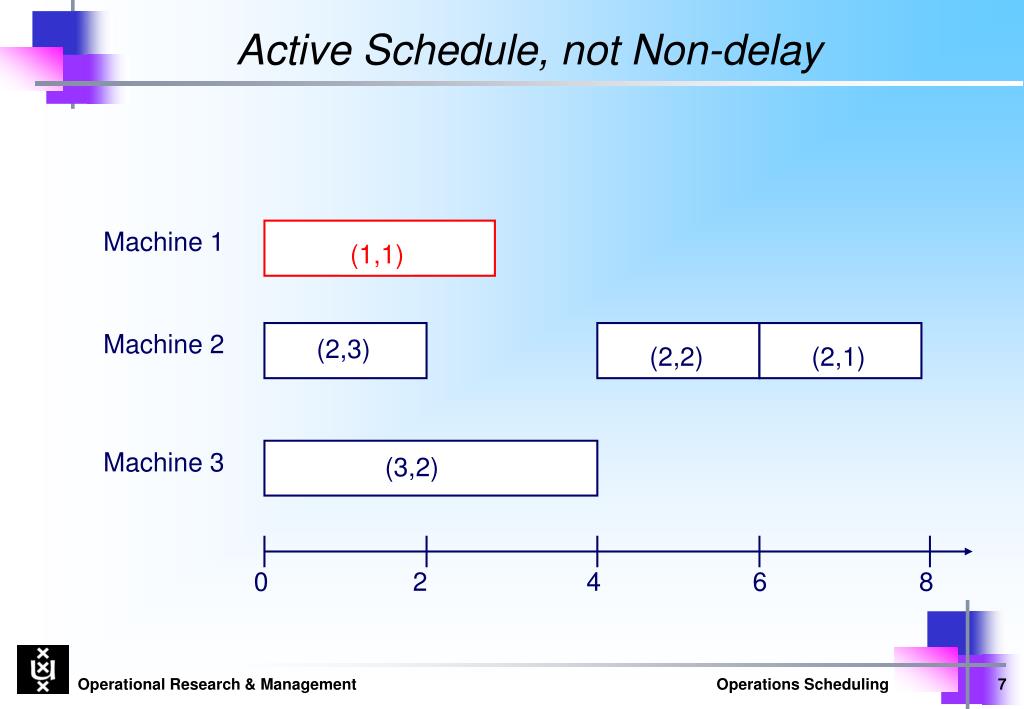
While this further reduces the search space, it comes with a risk: the optimal solution might not be a non-delay schedule. An active schedule may contain "beneficial" idle time, where a machine waits for a critical job to arrive, ultimately leading to a better overall makespan.

Role in Modern Metaheuristics

While the GT algorithm can be used as a standalone heuristic with a fixed priority rule, its real power in modern optimization lies in its use as a "schedule generator" or "decoder" within metaheuristics like Genetic Algorithms (GAs).

This is a key concept for your thesis work. Imagine a GA where a "chromosome" doesn't represent a full schedule, but rather a list of priorities or decisions. The GT algorithm can take this abstract representation and deterministically build a corresponding active schedule.

As the paper concludes, the key advantage is that "each solution is always a feasible and active schedule. Hence there is no repairing process required which can increase the efficiency of GA approach." This is a profoundly important technique in scheduling research. The complex search is handled by the metaheuristic, while the GT algorithm ensures that every candidate solution evaluated is valid and of high quality (i.e., active).

Conclusion

In this lesson, we transitioned from merely evaluating schedules to actively constructing them. The Giffler-Thompson algorithm provides a fundamental and elegant method for this task.

Key Takeaways:

• The set of active schedules is guaranteed to contain an optimal solution for makespan minimization, making it a valuable target for search algorithms.
• The Giffler-Thompson algorithm is an iterative procedure that constructs a single active schedule by resolving machine conflicts one at a time.
• At each step, the algorithm identifies a conflict set of operations competing for a machine, and a priority rule is used to select one.
• A slight modification to the algorithm generates non-delay schedules, a stricter subset that does not allow for deliberate machine idleness.
• In modern optimization, the GT algorithm is often used as a highly efficient decoder within metaheuristics (like Genetic Algorithms) to translate an abstract solution representation into a valid, active schedule.

Preview of the Next Lesson:

Having established a strong foundation in the classic Job Shop Problem—from its disjunctive graph representation and makespan calculation to the GT construction algorithm—we are now fully prepared to tackle the central topic of your thesis. In the next module, we will introduce the Flexible Job Shop Problem (FJSP). We will define this more complex environment and explore how the additional flexibility of machine choice transforms both the modeling and solution challenges.