Hello! Welcome to the first lesson in our module on Metaheuristics for Scheduling.
In our last module, we established a crucial point: realistic scheduling problems, especially the Flexible Job Shop Problem (FJSP) with setup and transport constraints, become computationally intractable for exact methods like MILP. The combinatorial explosion in complexity requires a different approach. This lesson marks our transition from exact optimization to the world of metaheuristics—powerful, intelligent strategies for finding high-quality solutions to these hard problems in a practical amount of time.
Our learning outcome for today is to analyze different neighborhood structures (e.g., swap, insertion) for local search. Local search is a fundamental metaheuristic concept, and the neighborhood structure is its most critical design component. Understanding how to define and analyze neighborhoods is the first step toward building sophisticated algorithms for your thesis research.
1. What is Local Search?
Local search algorithms are iterative improvement methods. They start with an initial solution and repeatedly try to find a better solution in the immediate vicinity, or "neighborhood," of the current one. This process focuses on exploitation (or intensification)—thoroughly searching a promising region of the solution space.
To get a clear picture of this core idea, please watch the first few minutes of the following video.
Introduction to Metaheuristics (7/9). Local search
This video from Luis R. Izquierdo provides an excellent introduction to the concept of local search. It explains the core idea of iteratively exploring a 'neighborhood' to find better solutions.
Please watch from the beginning to 04:57. Focus on: The general idea of starting with a solution and exploring its local neighborhood. The examples of how neighborhoods are defined for different solution representations (continuous, binary, and especially permutations).
As the video highlights, the central question in any local search algorithm is: How do you define the neighborhood? The answer depends entirely on how a solution is represented and the specific nature of the problem you are solving. For scheduling problems, where solutions are often represented as a permutation of jobs, we have a set of standard neighborhood operators.
2. Standard Neighborhood Structures for Permutation Scheduling
For a given job sequence (a permutation), a neighborhood is the set of all new sequences that can be reached by applying a specific "move" or "operator." Let's analyze the three most common ones.
The following paper provides clear, algorithm-style descriptions of these moves.
New effective neighborhoods for the permutation flow shop ...
The paper 'New effective neighborhoods for the permutation flow shop...' by Ben-Ammar et al. is a great resource. We will use it to formally define the standard neighborhood moves.
Please read Section 3.1, 'Description of the standard neighborhoods' (page 4-5). This section describes the Swap, Exchange, and Insertion moves. Pay attention to the simple pseudocode provided for each (Algorithms 3, 4, and 5).
Let's summarize and analyze these moves based on the reading. Consider a permutation of jobs.
a) Swap (or Adjacent Exchange)
This move consists of swapping two adjacent jobs in the sequence. For a sequence , a swap move at position results in the new sequence .
- Neighborhood Size: Since there are adjacent pairs, the neighborhood contains solutions. This is a relatively small neighborhood.
b) Exchange (or Pairwise Interchange)
This is a more general version of swap. It exchanges any two jobs at positions and . For a sequence , an exchange move results in the new sequence .
- Neighborhood Size: The number of neighbors is the number of ways to choose 2 jobs out of , which is . This is a much larger neighborhood, growing quadratically with the number of jobs.
c) Insertion (or Shift)
This move consists of taking a job from its current position and re-inserting it at another position . All jobs between positions and are shifted to make space.
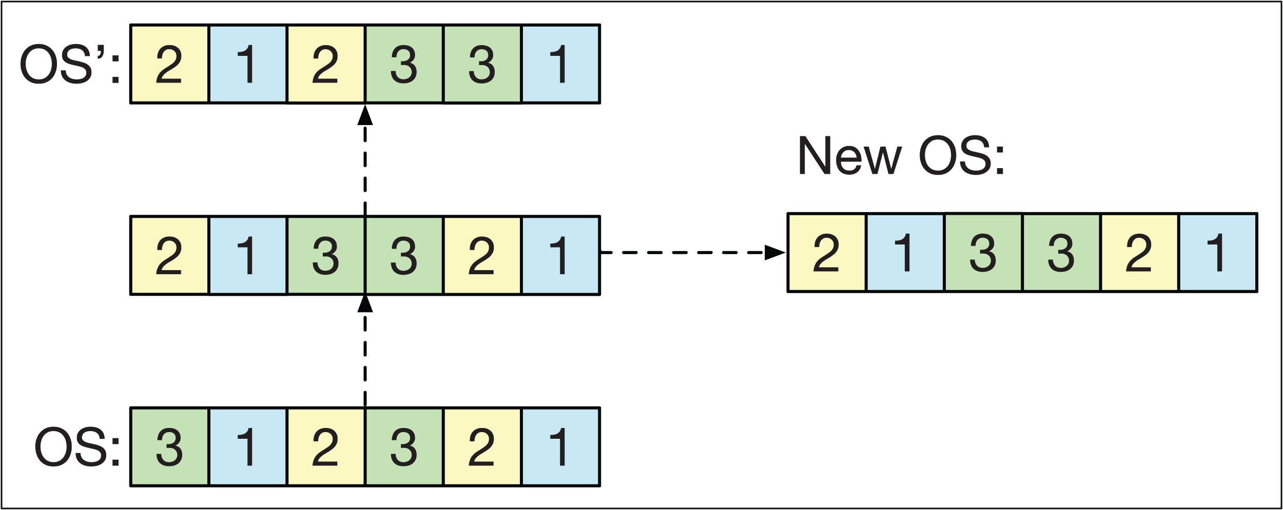
- Neighborhood Size: For each of the jobs, there are possible positions to insert it into. This gives a neighborhood size of . This is the largest of the three standard neighborhoods.
3. Analyzing and Comparing Neighborhoods
Choosing a neighborhood structure involves critical trade-offs. The "best" choice is not universal; it depends on the problem and the desired balance between search quality and computational speed.
Let's watch a short video segment that explains the importance of choosing a problem-appropriate neighborhood.
Introduction to Metaheuristics (8/9). Local search applied to the Travelling Salesman Problem
This second video from Luis R. Izquierdo discusses the concept of 'locality' and why the choice of neighborhood is not one-size-fits-all. It contrasts neighborhoods for the Traveling Salesman Problem (TSP) with those for permutation scheduling.
Please watch the segment from 06:08 to 09:13 and then from 11:52 to 15:29. Focus on: The concept of 'strong locality': neighbors should have similar quality (objective function values). Why a good neighborhood for TSP (2-opt) is not good for scheduling problems. Why Swap and Insertion moves are well-suited for scheduling problems (they preserve much of the relative job order).
Based on the resources, we can analyze the neighborhoods using three key criteria:
- Size & Computational Cost: A larger neighborhood offers more paths for improvement but takes longer to explore. Evaluating a single move (e.g., calculating the new makespan) also has a cost. For a flow shop with jobs and machines, a naive makespan calculation takes time. Thus, exploring a full Exchange neighborhood would take roughly , which is very slow. Clever acceleration techniques, like those developed by Taillard for the Insertion move, can reduce the cost of exploring the entire neighborhood to , making it much more practical.
- Locality & Solution Quality: As the video explained, good neighborhoods for scheduling should have strong locality. This means a small change to the sequence should result in a small change to the makespan. Swap and Insertion moves do this well because they preserve most of the relative ordering of jobs. Moves that drastically reorder the sequence (like the 2-opt for TSP) have weak locality for scheduling and lead to a very rugged, difficult-to-search landscape. Generally, larger neighborhoods (like Insertion) can navigate around local optima that would trap smaller neighborhoods (like Swap), leading to better final solutions.
- Connectivity of the Search Space: A neighborhood structure must ensure that it's possible to get from any solution to any other solution through a series of moves. All three structures we've discussed (Swap, Exchange, Insertion) guarantee this. A local search is guaranteed to find the global optimum if it starts from every possible solution. However, this is not a practical approach.
Here is a summary of the trade-offs:
| Neighborhood | Size | Typical Exploration Cost (without acceleration) | Solution Quality |
|---|---|---|---|
| Swap | Low (prone to getting stuck in poor local optima) | ||
| Exchange | Good | ||
| Insertion | (can be ) | Very Good (often considered the best for PFSP) |
Test your understanding!
In an Iterated Local Search (ILS) algorithm, a local search is run many times from different starting points. Given the trade-offs in the table above, which neighborhood structure—Swap or Insertion—might you choose if you only have a very limited time budget to run your entire ILS algorithm? Why?
Show answer
You would likely choose the Swap neighborhood.
Although the Insertion neighborhood generally leads to better-quality local optima, exploring it is computationally more expensive. With a very tight time budget, you can perform many fast local searches using the small Swap neighborhood. The hope is that by starting from many different points (the "iterated" part of ILS), you will stumble upon a region that contains a high-quality solution, even if the local search itself isn't as powerful. In contrast, running a single, slow local search with the Insertion neighborhood might exhaust your time budget before you can explore diverse regions of the search space. This is a classic example of the trade-off between the quality of a single search and the quantity of searches you can perform.
4. Neighborhoods for the Flexible Job Shop Problem (FJSP)
Your thesis focuses on the FJSP, which is more complex than a standard permutation flow shop. In FJSP, a solution is not just a single permutation; it involves two components:
- Machine Assignment (Routing): Assigning each operation to one of its eligible machines.
- Operation Sequencing: Ordering the operations assigned to each machine.
Therefore, neighborhood structures for FJSP must be designed to modify one or both of these components. The simple moves we've discussed are used as building blocks.
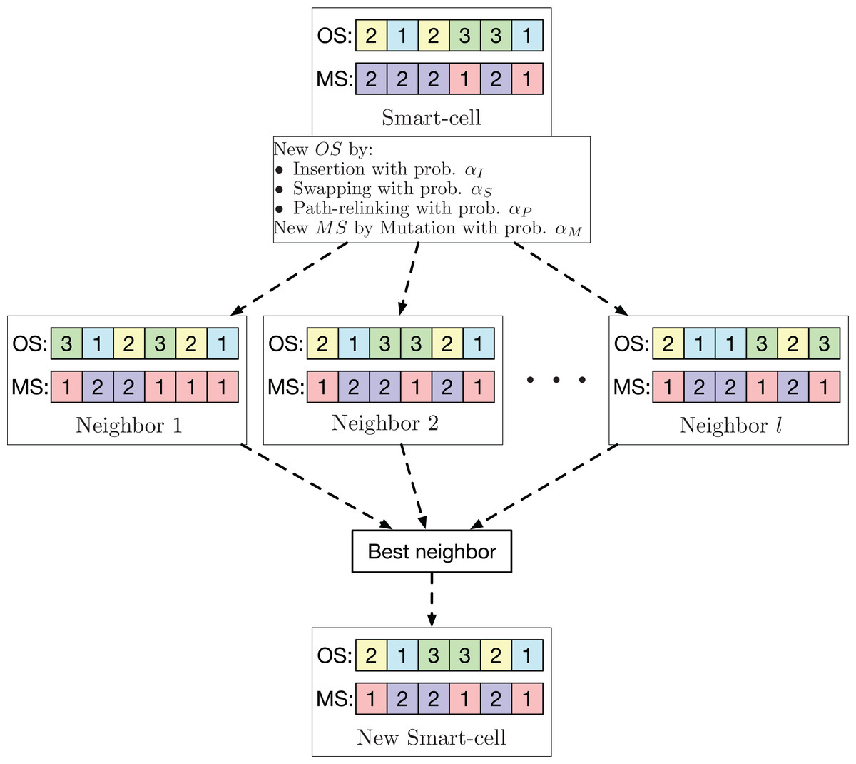
To see how this works in practice, let's examine a research paper that designed neighborhood moves specifically for FJSP.
A hybrid iterated local search metaheuristic for the flexible ...
The paper 'A hybrid iterated local search metaheuristic for the flexible...' by Cota et al. develops an algorithm for the FJSP. We will look at how they designed their neighborhood structures to handle both sequencing and machine assignment.
Please read Section A.4, 'Neighborhood Structures' (page 4). This section describes three neighborhood moves, N1, N2, and N3, used in their algorithm. Analyze what each move does and which part of the FJSP solution it targets (sequencing or routing).
From the paper, we can see a clear strategy for adapting neighborhood moves to the FJSP:
- N1 (Sequencing Move): This is a simple swap move on a randomly selected machine. It modifies the operation sequence on that machine but does not change any machine assignments.
- N2 (Routing Move): This move specifically targets flexibility. It takes an operation that can be processed on multiple machines and moves it to a different eligible machine. This modifies the machine assignment.
- N3 (Advanced Sequencing Move): This is a more complex version of an exchange move that also considers job precedence constraints. It modifies the operation sequence.
In a typical local search for FJSP, these different types of moves are often combined. At each step, the algorithm might randomly choose whether to apply a sequencing move (like N1 or N3) or a routing move (like N2) to generate a neighbor. This allows the search to explore changes in both dimensions of the problem simultaneously.
Conclusion
This lesson has served as your entry point into the practical world of metaheuristics. We have moved from why we need heuristics to how we start building them.
Key Takeaways:
- Local search improves a solution by exploring its neighborhood. The definition of this neighborhood is a critical design choice.
- For permutation-based scheduling, the most common neighborhood moves are Swap, Exchange, and Insertion.
- Analyzing a neighborhood involves evaluating its size, the computational cost of exploring it, and its locality (the ability to produce high-quality solutions). There is a fundamental trade-off between search speed and solution quality.
- For complex problems like FJSP, neighborhood structures are designed to modify different parts of the solution, such as the machine assignment (routing) and the operation sequence.
Preview of the Next Lesson:
Now that we know how to generate a neighborhood of solutions, the next logical question is: how do we select a neighbor to move to? And how does this choice influence the overall behavior of our search? In the next lesson, we will address this by exploring different local search strategies (like "first improvement" vs. "best improvement") and begin to evaluate the trade-off between exploration and exploitation in metaheuristic design.