Constraints, Complexity, and Model Size

1. The Challenge of Realism

Adding sequence-dependent setup times and transport constraints makes our models far more applicable to real-world industrial environments. However, this realism comes at a steep computational cost. These constraints don't just add a few new equations; they fundamentally change the nature and scale of the problem.

Let's break down this impact into two key areas:

1. Problem Complexity: The growth of the search space and the inter-dependencies between decisions.
2. Model Size: The corresponding increase in the number of variables and constraints in our mathematical formulation.

2. Impact on Problem Complexity

The core difficulty comes from a combinatorial explosion and a dense web of dependencies.

Combinatorial Explosion

A standard FJSP already involves two layers of decisions for each operation:

• Machine Assignment (Routing): Which machine should perform this operation?
• Operation Sequencing: In what order should operations assigned to the same machine be processed?

Adding setup and transport constraints adds new layers of decisions:

• Sequence-Dependent Setups: The sequencing decision now has direct time and cost implications, making the order itself a critical variable, not just a matter of feasibility.
• Transport Constraints: This can add two more decision layers:
  • Vehicle Assignment: Which transport vehicle (e.g., AGV) should move the job?
  • Vehicle Sequencing: In what order should a vehicle perform its assigned transport tasks?

Each new layer of choice doesn't just add to the complexity—it multiplies it. The total number of possible schedules grows exponentially, making an exhaustive search impossible for all but the smallest problems.

The Web of Dependencies

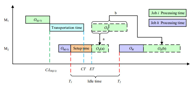
More importantly, these decisions are not independent. The optimal choice for one depends on the choices made for others, creating a tightly coupled system. Consider the start time of an operation $O_{ji}$. It cannot begin until a confluence of resources is available:

• The preceding operation of the same job, $O_{j,i-1}$, must be finished.
• The job must be physically present at the machine, meaning its transport task is complete.
• The assigned machine must be free, meaning the operation previously scheduled on it is finished.
• The setup for $O_{ji}$ must be completed, which can only start after the machine is free and its duration depends on the preceding operation on that machine.
• The assigned transport vehicle must be available to bring the next job.

This creates a complex chain of dependencies that is difficult for solvers to untangle. A small delay in one transport task can ripple through the schedule, delaying multiple machines and other jobs.

3. Impact on MILP Model Size

This increase in conceptual complexity translates directly into larger and more difficult MILP models.

• Variable Inflation:

  • To model sequence-dependent setups, we need binary variables (e.g., $z_{op1,op2,m}$) to capture the precedence of every pair of operations on a given machine. For $N$ operations and $M$ machines, this can introduce a number of variables on the order of $O(N^2\cdot M)$.
  • To model a fleet of transport vehicles, we need variables for vehicle assignment, start/end times of each transport task, and sequencing variables for each vehicle.

• Constraint Inflation:

  • Every new variable requires constraints to define its behavior.
  • The classic disjunctive constraints for machine sequencing must be modified to include the setup time parameter, linking the sequencing variables to the timeline.
  • New sets of disjunctive constraints are needed for each transport vehicle.
  • Crucial linking constraints must be added to connect the production schedule with the transport schedule (e.g., an operation's processing can only start after its transport is finished: $T^{start\_process}\ge T^{end\_transport}$).

This inflation in variables and constraints dramatically increases the memory required and the size of the solution space that the solver's branch-and-bound algorithm must explore.

4. Case Study: Deconstructing a Research Model

To see these impacts in a real, research-grade context, we will analyze a paper that models a highly complex system with both AGV transport and sequence-dependent setup times. This is an excellent example of the type of model relevant to your thesis.

Let's analyze what this paper reveals about complexity.

1. Model Components and Their Impact:
The model is rich with features that increase complexity:

• Flexible Flow Shop: Multiple parallel machines at each stage.
• AGVs: One transport vehicle between each stage.
• Sequence-Dependent Setup Times: explicitly modeled.
• Learning Effect: A sophisticated feature where setup times decrease with repetition, making the setup duration dependent on the entire history of operations.
• Energy Consumption: A second objective function, which is broken down into five components (Eq. 2-7), including specific terms for setup energy (ECSM) and transport energy (ECLM and ECNM).

Each of these features requires dedicated variables and constraints, as you saw in the formulation. For example, Constraints (16), (22), (23), and (24) are all dedicated to managing the timing of the AGVs. Constraints (17) and (18) model the complex setup time with a learning effect. The model size and complexity are clearly far greater than in a simple FJSP.

2. The Proof: Computational Limits
The most telling evidence of the impact of these constraints is in the computational results. Take a close look at Table 12.

• The authors use an exact method, AUGMECON, to solve the MILP for small problem instances.
• For PN1 (3 jobs, 3 stages), it finds an optimal solution in 2820 seconds (~47 minutes).
• For PN3 (7 jobs, 3 stages), the time balloons to 12,418 seconds (~3.5 hours).
• For PN4 (10 jobs, 3 stages) and larger, the solver times out after 14,400 seconds (>4 hours) without finding a solution.

This is a stark demonstration of NP-hardness in action. Adding just a few jobs makes the problem computationally intractable for an exact solver. The combinatorial explosion driven by the complex setup and transport decisions makes it impossible to prove optimality in a reasonable timeframe. This is the primary reason why researchers (and you, for your thesis) turn to heuristics and metaheuristics like NSGA-II, which the authors also use.

5. A Deeper Look at Complexity and Solution Space Structure

The size of the model is not the only factor. The very structure of the feasible region can make a problem difficult. Another research paper offers a fascinating insight into this.

The authors make a surprising discovery:

"First, and surprisingly, we can see that CPO consistently finds a schedule only for the general dataset F, but not for the present dataset P, although the latter is decomposable and involves fewer variables, constraints, and choices."

They reason that the more constrained problem (P) has a sparse and disconnected solution space, making it difficult for the solver to even find a valid starting point. The more flexible problem (F), despite having a larger search space, has a denser, more connected feasible region, making it easier for the solver to navigate.

This teaches us a valuable lesson: complexity is not just about size. The nature of the constraints and how they shape the geometry of the solution space is equally critical. Highly restrictive setup or transport rules might create a "brittle" problem that is harder to solve than a more flexible one.

Conclusion

In this lesson, we have dissected the profound impact of incorporating realistic setup and transport constraints into scheduling models. This analysis concludes our module on modeling and sets the stage for the rest of the course.

Key Takeaways:

• Combinatorial Explosion: Setup and transport constraints add multiple layers of decisions (sequencing, vehicle assignment, etc.), causing the search space to grow exponentially.
• Dense Dependencies: These constraints create a tightly coupled system where decisions about machines, jobs, and vehicles are all interdependent, making optimization extremely difficult.
• Model Inflation: The conceptual complexity translates into larger MILP models with significantly more variables and constraints.
• Intractability: As demonstrated by the case study, exact methods like MILP solvers fail to solve even moderately sized problems with these features within a practical timeframe.

Preview of the Next Module:

The intractability of exact models for complex, real-world FJSP is the primary motivation for turning to approximation methods. We cannot guarantee optimality, but we can aim to find very good solutions in a reasonable amount of time. In our next lesson, we will begin Module 8: Metaheuristics for Scheduling. We will start with the fundamental building blocks of many powerful algorithms by learning to analyze different neighborhood structures for local search.