Flexible Job Shop Scheduling with Setup and Transport Constraints

Hello! Welcome to the final lesson in our module on modeling complex constraints.

In our last two sessions, we tackled sequence-dependent setup times and transportation constraints separately, building a MILP for each. You saw how to model the logic of machine changeovers and how to formulate an integrated problem that schedules both machines and a fleet of transport vehicles.

Today, we will synthesize these two concepts. Our learning goal is to formulate a flexible job shop MILP that includes both setup and transport constraints. This represents a comprehensive and realistic model of a modern manufacturing system. Mastering this will provide you with a powerful tool for your thesis research, allowing you to model the complex, interacting systems that are central to the Flexible Job Shop Problem.

We will proceed in two main steps. First, we'll examine a published MILP model that integrates both constraint types in a specific way. Second, we will discuss how to conceptually construct a more general model by merging the formulations from our previous lessons.

1. The Interplay of Setups and Transports

Before diving into the mathematics, let's establish a clear picture of how these constraints interact. An operation can only begin when two conditions are met:

The required machine is ready. This means the previous operation on that machine is finished, and the necessary setup for the new operation has been completed.
The required job is present. This means the transport task to bring the job from its previous location to the current machine has been completed.

The start time of any given operation is therefore constrained by both the machine's schedule and the transport schedule. A Gantt chart helps visualize this sequence of dependencies.

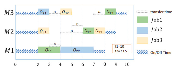
Gantt Chart Illustrating Job Scheduling with Transfer and On/Off Times — This Gantt chart illustrates the key time components we need to model. An operation (e.g., Job 2's second operation on M2) can only start after the previous operation on that machine is done, a setup ('On/Off Time') is performed, and the job itself has arrived ('transfer time'). Our MILP must manage all these dependencies.

As you can see, the 'transfer time' must finish before the 'On/Off Time' (setup) can even be considered useful. A machine could be free and ready, but if the job hasn't arrived, it sits idle. Conversely, a job could be waiting at a machine that is still busy processing or being set up after a previous job.

2. An Integrated MILP Formulation

Different researchers have modeled this combined problem in various ways. The exact formulation often depends on the specific characteristics of the transport system. Let's analyze one such model that handles sequence-dependent setups and a specific type of transport constraint based on the physical layout of the workshop.

Flexible job shop scheduling problem with sequence-dependent transportation constraints and setup times

The paper 'Flexible job shop scheduling problem with sequence-dependent transportation constraints and setup times' by Varone, Schindl, and Beffa presents a MILP for this exact problem. Please read the sections detailing the model's structure.

Please read Section III.A ('Variables') to understand the decision variables used. Then, carefully review Section III.B ('Constraints'). You don't need to absorb every equation, but focus on identifying how and where setup times and transport logic are incorporated.

This model provides a complete formulation that integrates both constraint types. Let's dissect the key components.

Key Variables

The model uses the standard variables you're familiar with:

$x_{j, O_{j l}}$ : The continuous variable for the start time of operation $l$ of job $j$ .
$y_{j, O_{j l}, m}$ : A binary variable, 1 if operation $l$ of job $j$ is assigned to machine $m$ .
$z_{j_{1}, O_{j_{1} l_{1}}, j_{2}, O_{j_{2} l_{2}}}$ : A binary variable, 1 if the operation for job $j_{1}$ precedes the operation for job $j_{2}$ .

Integrating Setup Times

The model cleverly integrates sequence-dependent setup times into the core precedence constraints. Notice the parameter prep, which stands for preparation time. In this paper, it's a function of machine temperature, but you can think of it as a general setup time $s (o p_{p r e v}, o p_{c u r r}, m)$ .

Constraint 4) "No conflict on the same machine":
This is the classic disjunctive constraint for two operations, $(j_{1}, l_{1})$ and $(j_{2}, l_{2})$ , on the same machine $m$ . The formulation ensures that if $(j_{2}, l_{2})$ precedes $(j_{1}, l_{1})$ , then:
$x_{j_{1}, O_{j_{1}, l_{1}}} \geq x_{j_{2}, O_{j_{2}, l_{2}}} + p_{O_{j_{2}, l_{2}}} + prep_{T_{e, j_{2}}, T_{b, j_{1}}, m}$
This directly enforces that the start time of the next operation must accommodate the processing time of the previous operation plus the required setup time. This is the core mechanism for modeling sequence-dependent setups.

Integrating Transport Constraints

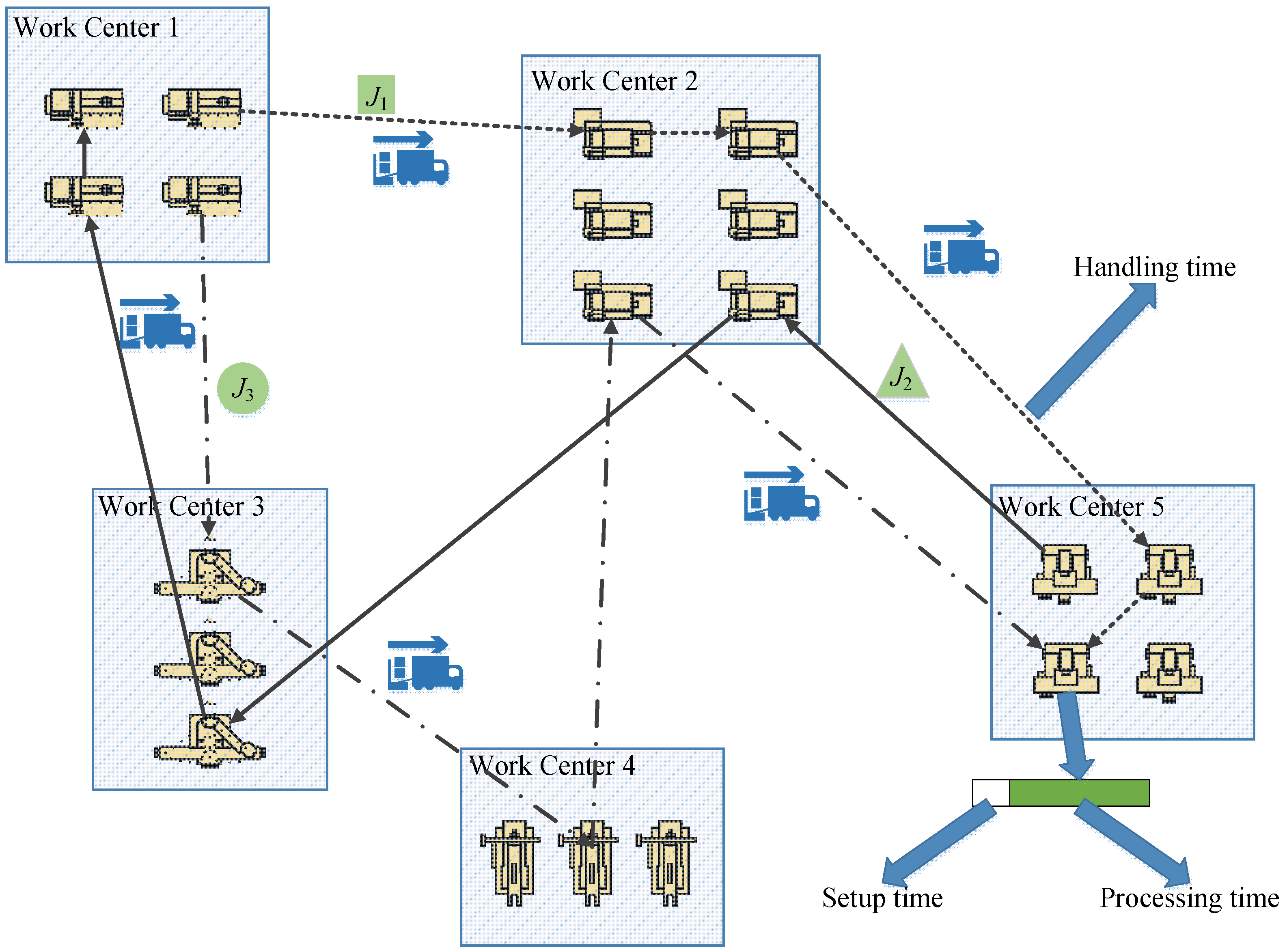
This paper models transport in a way that differs from the vehicle-fleet approach we saw last lesson. It uses layout-based or topological constraints:

Constraint 11) "Impossible machine successions":
$y_{j, O_{j l}, m_{1}} + y_{j, O_{j l + 1}, m_{2}} = 0 \forall (m_{1}, m_{2}) \in incompatibleSuccession$
This is a simple but effective way to model physical transport limitations. It states that if moving from machine $m_{1}$ to $m_{2}$ is impossible (e.g., no connecting conveyor belt), then no job can have consecutive operations assigned to that machine pair.
Constraint 12) "Blocking operation":
This is a more sophisticated transport constraint. It models scenarios where an operation running on one machine ( $m_{i}$ ) can physically block the path for a job moving between two other machines ( $m_{j}$ and $m_{k}$ ).

This modeling style is highly relevant for systems with fixed transport paths or spatial interference, whereas the vehicle-based model from our previous lesson is suited for systems with flexible movers like AGVs.

Flexible Job Shop Problem with Setup and Transport Considerations — This diagram shows jobs moving between work centers. The model from the paper we just reviewed is excellent for capturing constraints like 'the path from Work Center 1 to Work Center 3 is blocked if a large job is being processed in Work Center 4'.

3. Conceptually Building a Comprehensive Model

The paper gives us one complete example. Now, let's perform an exercise that is central to research: combining ideas from different models. How would we integrate sequence-dependent setup times into the vehicle-based transport model from our last lesson?

Recall the key constraints from that model (from paper A review of flexible job shop scheduling problems...):

Machine Sequencing:
$T_{j_{1} i_{1}}^{s p} - T_{j_{2} i_{2}}^{e p} \geq M (Y_{j_{1} i_{1}, j_{2} i_{2}}^{m} - 1)$
This says operation $(j_{1}, i_{1})$ must start after $(j_{2}, i_{2})$ finishes, if they are sequential on machine $m$ .
Transport-Production Link:
$T_{j i}^{s p} \geq T_{j i}^{e t}$
This says an operation can only start processing ( $T^{s p}$ ) after its transport is complete ( $T^{e t}$ ).

To add sequence-dependent setup times, we would introduce a parameter $s_{j_{2} i_{2}, j_{1} i_{1}, m}$ and modify the machine sequencing constraint:

$T_{j_{1} i_{1}}^{s p} - T_{j_{2} i_{2}}^{e p} - s_{j_{2} i_{2}, j_{1} i_{1}, m} \geq M (Y_{j_{1} i_{1}, j_{2} i_{2}}^{m} - 1)$

By making this single modification, the entire model is updated. The solver, in minimizing the makespan, must now find start times ( $T^{s p}$ ) that satisfy all the constraints simultaneously:

The job must have arrived (the transport constraint).
The machine must be free and the setup complete (the modified machine sequencing constraint).
The vehicle must be available (the vehicle sequencing constraints).

This demonstrates the power and modularity of MILP. By adding or modifying constraints, you can systematically increase the model's fidelity to the real-world problem you are studying for your thesis.

Test your understanding!

Imagine a scenario where setup can be done partially before the job arrives. For example, a technician can load new tool-holders onto a machine, but the final calibration (the last 5 minutes of the setup) can only be done once the actual job piece is loaded.

How would you conceptually adapt the MILP formulation to handle this "pre-setup" idea?

Show answer

This is an excellent question that pushes toward advanced modeling techniques. Here's a conceptual approach:

Split the Setup Time: The setup time parameter $s_{j^{'} i^{'}, j i, m}$ would be split into two parts:
- $s_{j^{'} i^{'}, j i, m}^{p r e}$ : The portion of the setup that can be done before the job arrives.
- $s_{j^{'} i^{'}, j i, m}^{p os t}$ : The portion that must be done after the job arrives.
Introduce a New Time Variable: We would need a new continuous variable, perhaps $T_{j i, m}^{p r e_se t u p_e n d}$ , representing the completion time of the pre-setup for operation $(j, i)$ on machine $m$ .
Modify the Constraints:
- The pre-setup can start as soon as the previous operation on the machine is done:
  $T_{j i, m}^{p r e_se t u p_e n d} \geq T_{j^{'} i^{'}}^{e p} + s_{j^{'} i^{'}, j i, m}^{p r e}$
- The final operation start time ( $T_{j i}^{s p}$ ) now depends on two events: the completion of the pre-setup AND the arrival of the job. The post-setup happens after both are done.
  $T_{j i}^{s p} \geq T_{j i, m}^{p r e_se t u p_e n d} + s_{j^{'} i^{'}, j i, m}^{p os t}$
  $T_{j i}^{s p} \geq T_{j i}^{e t} + s_{j^{'} i^{'}, j i, m}^{p os t}$
  These constraints ensure that the processing starts only after the pre-setup is done, the job has arrived, and the post-setup is completed. This adds complexity but also significant realism to the model.

Conclusion

In this lesson, we successfully combined two of the most critical real-world constraints into a single FJSP formulation. You have not only analyzed a formal MILP model from the literature but also reasoned through how to construct your own by merging concepts from previous lessons.

Key Takeaways:

Modeling an FJSP with both setup and transport constraints requires integrating machine-level sequencing with job and vehicle routing.
The core of the integration lies in ensuring an operation's start time respects both machine availability (after processing and setup) and job availability (after transport).
MILP provides a flexible framework where these different constraints can be layered together into a single, solvable model.
Transport constraints can be modeled explicitly (vehicle fleets, travel times) or implicitly/topologically (blocking rules, impossible paths), depending on the system's nature.

Preview of the Next Lesson:

We have reached the apex of what can be practically solved with exact MILP models. For the large-scale, complex FJSP instances you'll encounter in your research, these models become computationally intractable. Therefore, we must turn to advanced heuristics. In the next module, we will begin our exploration of Metaheuristics for Scheduling. Our first lesson will focus on the building blocks of these methods, starting with an analysis of different neighborhood structures for local search.

Recommended resources