Optimizing Schedules with Time and Resource Constraints

Hello! Welcome to the next lesson in our journey through complex scheduling problems.

In our previous session, we established the fundamental concepts of modeling transportation, distinguishing between simple time lags and the more realistic approach of modeling a finite fleet of transport resources. We defined key terms like empty vs. loaded travel and identified the new parameters and decision variables required.

Today, we will build directly on that foundation. The learning outcome for this lesson is to integrate transport time and resource constraints into scheduling models. We will move from conceptual definitions to a concrete mathematical formulation, focusing on how to construct a Mixed-Integer Linear Program (MILP) that simultaneously schedules both production and transportation. This is a critical skill for your thesis, as it allows you to create a comprehensive and solvable representation of the Flexible Job Shop Problem with Transport (FJSP-T).

1. The Integrated Scheduling Problem: FJSP with Transportation

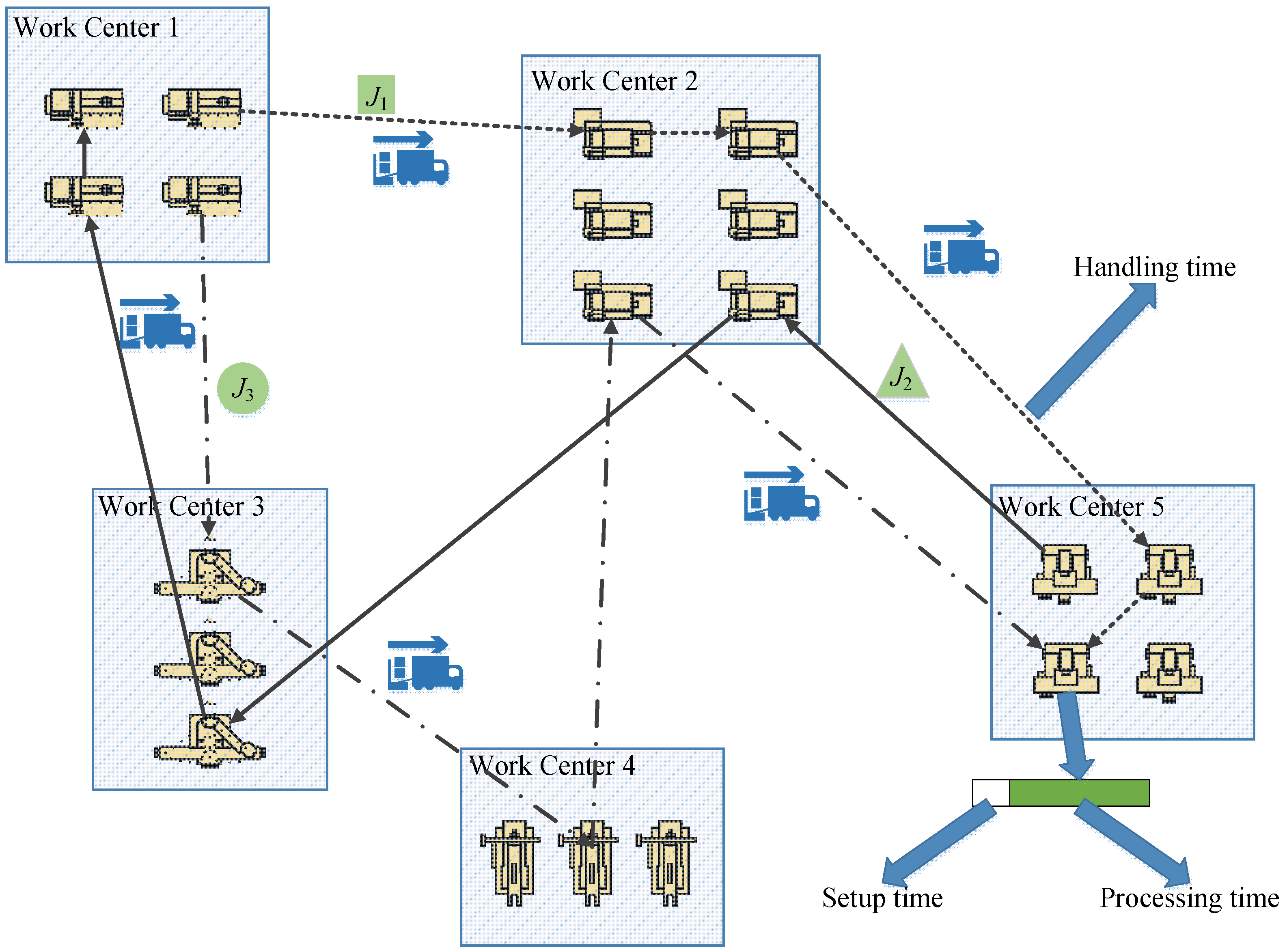
The problem we are tackling is a significant extension of the standard FJSP. By including a finite number of vehicles, we are essentially adding another layer of resource constraints. A job's operation cannot start until:

Its preceding operation is finished.
The machine it needs is free.
The job has been physically transported to that machine by an available vehicle.

This creates a tight coupling between the machine schedule and the vehicle schedule. To better understand this integrated problem, let's start with a formal definition from the literature.

A review of flexible job shop scheduling problems considering transportation vehicles

The paper 'A review of flexible job shop scheduling problems considering transportation vehicles' provides an excellent overview. Please read the introductory sections to solidify your understanding of the problem's context and complexity.

Please read Section 1 ('Introduction') and Section 2.1 ('Problem positioning'). Focus on how the authors describe the alternate occurrence of transportation and processing stages and the three essential subproblems: job routing, operation sequencing, and transportation task assignment.

As the paper highlights, solving this problem, which is often abbreviated as FJSP_PT, involves solving three interconnected subproblems. Our goal is to create a single mathematical model that finds an optimal solution for all three simultaneously.

Manufacturing System with Work Centers, Job Flow, and Time Components — This diagram illustrates a manufacturing system where jobs move between different work centers. The 'Handling time' indicated by the trucks represents the transport operations we are about to model. An effective schedule must coordinate the processing within each work center with the handling time between them.

2. A MILP Model for the FJSP_PT

Given your background in industrial engineering and mathematical analysis, you know that a MILP formulation is a powerful way to represent such complex optimization problems. We will now examine a complete MILP model for the FJSP_PT that aims to minimize makespan ( $C_{ma x}$ ).

This model will bring together concepts we've seen before (like sequencing variables for machines) and integrate the new transport-related variables from our last lesson.

A review of flexible job shop scheduling problems considering transportation vehicles

Now, let's dive into the mathematical details. Please study the integer programming model presented in the same review paper.

Carefully read Appendix A, which contains the full 'Integer programming model of FJSP_PT'. Familiarize yourself with the notation in Table A1 and skim through the constraints (A1) to (A24). Don't worry about understanding every detail immediately; we will break down the key transport-related constraints next.

3. Deconstructing the Transport Constraints

The model you just reviewed contains many constraints. Some of them, like (A3)-(A11), should look familiar as they handle the core machine assignment and sequencing aspects of the FJSP. Our focus will be on the new constraints, (A12) through (A21), which specifically model the transportation system.

Let's break them down by function.

a) Vehicle Capacity and Routing Constraints

These constraints manage the fleet of vehicles. They ensure we don't use more vehicles than are available and that each vehicle follows a valid sequence of tasks.

Constraint (A12): $\sum_{j \in J} \sum_{i \in O p r_{j}} U_{j i} \leq N A$
- Logic: The variable $U_{j i}$ is 1 if the transport task for operation $O_{j i}$ is the first task for some vehicle. The sum of all "first tasks" must be less than or equal to the number of available vehicles ( $N A$ ). This effectively limits the number of active vehicle routes.
Constraint (A13): $\sum_{j \in J} \sum_{i \in O p r_{j}} R_{j i} = \sum_{j \in J} \sum_{i \in O p r_{j}} U_{j i}$
- Logic: $R_{j i}$ is 1 if the transport task for $O_{j i}$ is the last task for a vehicle. This constraint ensures that every vehicle route that is started also has an end.
Constraints (A14) & (A15): These constraints use the sequencing variable $W_{j_{2} i_{2}, j_{1} i_{1}}^{k}$ (task for $O_{j_{1} i_{1}}$ follows task for $O_{j_{2} i_{2}}$ on vehicle $k$ ) to ensure that every transport task has exactly one predecessor and one successor within a vehicle's route (unless it's the first or last task). This is analogous to the machine sequencing constraints you've seen before.

b) Linking Transport Completion to Production Start

These are the most critical constraints, as they create the dependency between the transport system and the production system.

Constraint (A16): $T_{j i}^{e p} - T_{j i}^{e t} - t P_{j im} \geq M (X_{j i}^{m} - 1)$
- Logic: This is a "Big-M" constraint. If operation $O_{j i}$ is assigned to machine $m$ ( $X_{j i}^{m} = 1$ ), the right-hand side becomes 0. The constraint then enforces $T_{j i}^{e p} - T_{j i}^{e t} \geq t P_{j im}$ , which simplifies to $T_{j i}^{e p} \geq T_{j i}^{e t} + t P_{j im}$ .
- In words: The processing end time ( $T_{j i}^{e p}$ ) must be greater than or equal to the transport end time ( $T_{j i}^{e t}$ ) plus the processing time ( $t P_{j im}$ ). This ensures an operation doesn't start processing until the job has physically arrived.

c) Calculating Transport End Times

This final set of constraints determines the value of $T_{j i}^{e t}$ , the time a transport task is completed. This is where empty and loaded travel times come into play.

Constraint (A18) - Consecutive Operations of the Same Job: $T_{j i}^{e t} - T_{j (i - 1)}^{e p} - t_{m^{'} m}^{'} \geq M (X_{j i}^{m} + X_{j (i - 1)}^{m^{'}} - 2)$
- Logic: If $O_{j i}$ is on machine $m$ and its predecessor $O_{j (i - 1)}$ was on machine $m^{'}$ , this constraint becomes active. It states that the arrival time at machine $m$ ( $T_{j i}^{e t}$ ) must be after the completion time at machine $m^{'}$ ( $T_{j (i - 1)}^{e p}$ ) plus the loaded travel time between the machines ( $t_{m^{'} m}^{'}$ ). (Note: The paper seems to use $t^{'}$ for loaded time and $t$ for empty time, which can be counter-intuitive. Always check notation carefully!)
Constraints (A20) & (A21) - Consecutive Tasks on the Same Vehicle: These are the most complex constraints. They model the sequence of tasks for a single vehicle. Let's analyze the logic of (A20):
- Scenario: A vehicle completes the transport for operation $O_{j_{2} i_{2}}$ (which was processed on machine $m^{''}$ ) and its next task is to transport for operation $O_{j_{1} i_{1}}$ (which needs to go to machine $m$ ).
- Time Calculation: The arrival time for the new task ( $T_{j_{1} i_{1}}^{e t}$ ) depends on the arrival time of the previous task ( $T_{j_{2} i_{2}}^{e t}$ ) plus two travel components:
  1. Empty Travel: From the drop-off location of the previous task ( $m^{''}$ ) to the pickup location of the new task ( $m^{'}$ , where $O_{j_{1} (i_{1} - 1)}$ was processed). This is $t_{m^{''} m^{'}}$ .
  2. Loaded Travel: From the pickup location ( $m^{'}$ ) to the drop-off location ( $m$ ). This is $t_{m^{'} m}^{'}$ .
- The constraint combines these pieces to correctly calculate the transport end time based on vehicle availability and travel distances.

Test your understanding!

Consider constraint (A18) from the paper: $T_{j i}^{e t} - T_{j (i - 1)}^{e p} - t_{m^{'} m}^{'} \geq M (X_{j i}^{m} + X_{j (i - 1)}^{m^{'}} - 2)$ .

Suppose in a real factory, some jobs are very heavy and require a special, slower type of vehicle, while other jobs are light and can be moved by faster vehicles. The current model assumes all travel times ( $t^{'}$ ) depend only on the origin and destination machines.

How would you need to modify the model's parameters and this constraint to account for job-dependent (and thus vehicle-dependent) travel times?

Show answer

To handle this, you would need to make the travel time parameter more specific.

Modify the Parameter: Instead of $t_{m^{'} m}^{'}$ , you would need a parameter like $t_{m^{'} mj}^{'}$ or $t_{m^{'} m c}^{'}$ , representing the loaded travel time between machines $m^{'}$ and $m$ for job $j$ or for a job of class $c$ . If it depends on the specific vehicle type, you might even need $t_{m^{'} mk}^{'}$ for vehicle $k$ . Let's assume it's job-dependent: $t_{m^{'} mj}^{'}$ .
Modify the Constraint: The constraint itself would be updated to use this more specific parameter:
$T_{j i}^{e t} - T_{j (i - 1)}^{e p} - t_{m^{'} mj}^{'} \geq M (X_{j i}^{m} + X_{j (i - 1)}^{m^{'}} - 2)$
This change ensures that when calculating the arrival time for job $j$ , the model uses the correct travel time associated with that specific job. This highlights how these MILP models can be extended to capture more nuanced, real-world details, which is a key part of academic research in this area.

Conclusion

In this lesson, we successfully bridged the gap from concept to implementation by integrating transportation constraints directly into a MILP model for the Flexible Job Shop Problem. You have seen how to formulate the problem to simultaneously optimize machine and vehicle schedules.

Key Takeaways:

The FJSP with transport resources (FJSP_PT) is an integrated problem requiring the simultaneous solution of machine assignment, machine sequencing, vehicle assignment, and vehicle sequencing.
A MILP model can capture all these decisions using binary variables for assignment and sequencing, and continuous variables for event times.
The key to the integration lies in the linking constraints, which ensure that a production operation can only start after the transport task delivering the job has been completed.
Calculating transport completion times is complex, as it must account for vehicle availability, the vehicle's previous location (for empty travel), and the job's current location (for loaded travel).

Preview of the Next Lesson:

You have now modeled sequence-dependent setups and transportation constraints separately. The final step in this module is to combine them. In our next lesson, we will focus on formulating a flexible job shop MILP that includes both setup and transport constraints. This will result in a highly comprehensive and realistic model, representing the state-of-the-art for many industrial applications and providing a strong foundation for the models in your thesis.

Recommended resources