Hello! Welcome back to our course.
In our last session, we focused on modeling complexities that occur on a machine, specifically sequence-dependent setup times. We saw how to integrate these into both disjunctive graph and MILP models to capture the time cost of changing from one job to another.
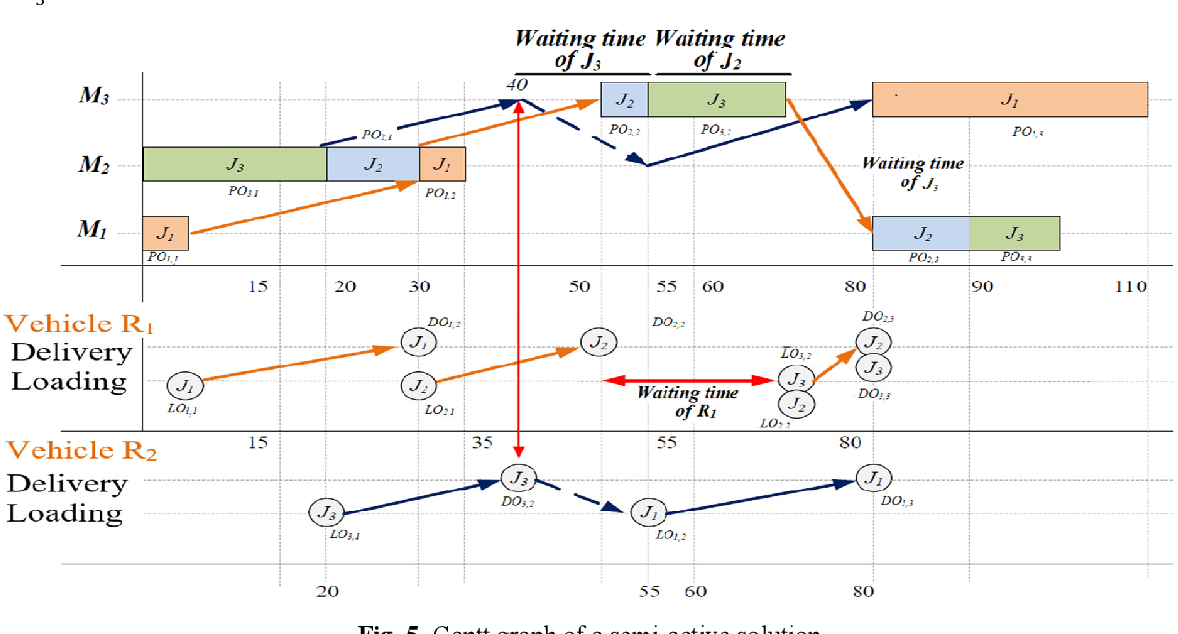
Today, we shift our focus to what happens between machines. In any realistic production facility, jobs don't teleport; they are moved by resources like Automated Guided Vehicles (AGVs), forklifts, or conveyors. The goal of this lesson is to learn how to define transport constraints and model these transport resources. This is a crucial step in building the comprehensive and realistic Flexible Job Shop Problem (FJSP) models that will be central to your thesis work.
1. From Idealized Transport to Realistic Constraints
In introductory scheduling models, transportation is often either ignored or heavily simplified. As your work requires a high degree of academic rigor, it's essential to understand the different levels of modeling transport and why a detailed approach is necessary.
The best way to see this is to compare different problem definitions. A research paper by Berterotti`ere et al. offers a clear way to categorize these problems.
Flexible job-shop scheduling with transportation resources
To understand the different ways to model transport, please examine 'Table 1: Comparison of FJSP with transportation resources with simpler problems' in the paper 'Flexible job-shop scheduling with transportation resources'. This table provides an excellent summary.
Locate 'Table 1' near the beginning of Section 3. Pay close attention to the last two rows, which distinguish between modeling 'transportation times' and 'transportation resources'.
As the table illustrates, we can distinguish between two main ways of considering transport:
-
FJSP with Transportation Times (Time Lags): This approach adds a fixed or machine-dependent travel time between consecutive operations of a job. For example, after an operation on Machine A finishes, a delay of is added before the next operation can start on Machine B. The critical assumption here is that a transportation resource is always available the instant it's needed. This is often unrealistic, as it implies an infinite number of vehicles, which is costly and would lead to congestion.
-
FJSP with Transportation Resources (FJSPT): This is the more realistic and complex model that we will focus on. It explicitly models a finite fleet of vehicles (e.g., AGVs). This means transportation itself becomes a scheduled activity. This model decomposes the problem into several interdependent subproblems, including:
- Machine Assignment: Assigning a production operation to an eligible machine.
- Operation Sequencing: Sequencing the operations assigned to each machine.
- Vehicle Assignment: Assigning a transport task to an available vehicle.
- Vehicle Routing/Scheduling: Sequencing the transport tasks for each vehicle.
By modeling transport resources explicitly, we acknowledge that vehicles are a bottleneck and their availability directly impacts the production schedule.

2. Defining Transport Operations and Resources
To model the FJSPT, we need to formalize the components of the transportation system. Let's define the key concepts, drawing from the formal problem description found in scheduling literature.
A transport operation is initiated when a job finishes a production operation (operation of job ) on machine and needs to move to machine for the next production operation, .
This process involves two key phases for the vehicle:
- Empty Travel: The vehicle, currently located where it finished its last task (e.g., at machine ), travels empty to the pickup location, machine . The time for this depends on the distance between and .
- Loaded Travel: The vehicle picks up the job at machine and transports it loaded to the drop-off location, machine . The time for this depends on the distance between and .
A key assumption often made in this context, which is quite realistic, is that travel times satisfy the triangular inequality: the time to travel from A to B is always less than or equal to the time to travel from A to C and then from C to B.
This explicit handling of transport introduces significant dependencies. A job can't start processing on a machine until it physically arrives, and its arrival time depends on:
- When its previous operation was completed.
- When a vehicle was assigned to transport it.
- The vehicle's location prior to the task (determining empty travel time).
- The travel time from the pickup to the drop-off machine (loaded travel time).
A MILP Model for Energy-Efficient Job Shop Scheduling ...
For a formal definition of these concepts, let's turn to the paper 'A MILP Model for Energy-Efficient Job Shop Scheduling ... and Transport Resources' by Homayouni and Fontes. It provides a very clear description of the transport system.
Please read Section 2, 'Problem Definition'. Focus on the paragraphs describing the 'transport system'. This will reinforce the concepts of identical vehicles, the LU (load/unload) area, and empty vs. loaded travel.
3. Key Parameters and Variables for Modeling Transport
Now that we have defined the concepts, let's see how they are translated into a mathematical model. While the full MILP integration is the topic of our next lesson, we can already define the necessary building blocks: the parameters and decision variables.
Based on your background in mathematical analysis, you'll recognize this as the first step in formulating any optimization problem. We'll again refer to the model by Homayouni and Fontes as it lays out these components very clearly.
Key Parameters (Inputs to the model)
- : The number of available vehicles in the fleet.
- : The empty travel time for a vehicle to move from the location of task 's drop-off to the location of task 's pick-up.
- : The loaded travel time required for transport task . This is the time to move the job from its origin machine to its destination machine.
Key Decision Variables (Outputs of the model)
- : A continuous variable representing the arrival time of the job for operation at its designated machine. This is a critical variable connecting the transport and production schedules.
- : A binary variable that equals 1 if transport task is performed by the same vehicle immediately after transport task . This variable establishes the sequence, or route, for each vehicle.
- : A binary variable that equals 1 if transport task is the first task performed by any vehicle.
Using these variables, we can formulate constraints that govern the transport system. For example:
- Vehicle Capacity: The number of vehicle routes (i.e., the number of tasks designated as a "first task") cannot exceed the total number of available vehicles ().
- Job Arrival Time: A production operation (with predecessor ) cannot start before the job arrives. The arrival time must be greater than or equal to the completion time of the previous operation plus the loaded travel time .
- Vehicle Continuity: If a vehicle performs task right after task , its arrival at the destination for task depends on when it arrived at its destination for task (), plus the empty travel time () and loaded travel time () for the new task. This creates a "no-overlap" constraint for vehicles.
(Note: This is a simplified representation of constraint (14) in the paper, which uses the "big-M" method to activate it only when .)
Test your understanding!
Let's consider a simple scenario:
- Operation of Job 1 finishes on Machine M1 at time .
- The next operation, , must be processed on Machine M2.
- A single vehicle, AGV1, is available to transport the job. AGV1 just completed a task and is now idle at Machine M3, becoming free at time .
- Travel times are as follows:
- Empty travel from M3 to M1: 4 minutes.
- Loaded travel from M1 to M2: 6 minutes.
Answer the following questions:
- When does AGV1 arrive at M1 to pick up the job?
- When does the job physically arrive at M2?
- What is the earliest possible start time for operation ?
Show answer
-
AGV1 Arrival at M1:
- AGV1 is free at M3 at time 15. The travel to M1 takes 4 minutes. So, it could arrive at M1 at time .
- However, the job at M1 is only ready to be picked up at time 20.
- Therefore, the AGV arrives at M1 at time 19 but must wait. The actual pickup occurs at .
-
Job Arrival at M2:
- The AGV picks up the job at M1 at time 20.
- The loaded travel from M1 to M2 takes 6 minutes.
- Therefore, the job arrives at M2 at time .
-
Earliest Start Time for :
- Since the job is not physically present at M2 until time 26, operation cannot begin before this time, even if M2 is idle. So, the earliest possible start time is .
Conclusion
In this lesson, you have learned to define and conceptualize transport constraints in a flexible job shop environment. This is a significant step up from simplified models and is essential for creating scheduling models that reflect real-world logistics.
Key Takeaways:
- Modeling transportation resources (like a finite fleet of AGVs) is more realistic than using simple transportation times (time lags), as it accounts for vehicles being a limited, shared resource.
- This introduces new scheduling decisions: vehicle assignment (which vehicle takes which job) and vehicle routing (the sequence of tasks for each vehicle).
- The total transport time for a single job movement consists of two parts: the empty travel of the vehicle to the pickup location and the loaded travel to the drop-off location.
- We can begin to model these constraints mathematically by defining specific parameters (travel times, fleet size) and decision variables (vehicle sequences, job arrival times).
Preview of the Next Lesson:
We have now defined all the necessary components for both sequence-dependent setups and transportation. In our next lesson, we will put everything together and focus on how to integrate transport time and resource constraints into scheduling models. We will explore how to extend the disjunctive graph to include vehicle resources and how to write the complete MILP constraints that simultaneously solve for the production and transportation schedules.