Flow Shop Scheduling: Implementing Swap-Based Local Search

Hello! Welcome to our next lesson on heuristics for the flow shop problem.

In our last session, we focused on the NEH heuristic, a powerful constructive method that builds a high-quality schedule from scratch. We saw how its principle of prioritizing jobs with high total processing times leads to very effective solutions.

However, constructing a good solution is often just the first step. The natural next question is: can we take a good solution and make it even better? This brings us to the world of improvement heuristics. Today, we will explore the most fundamental improvement technique: local search.

Our learning outcome is to implement a swap-based local search procedure for flow shop schedule improvement. This is a critical concept, as local search is the foundation for nearly all advanced metaheuristics (like Tabu Search, Simulated Annealing, and Genetic Algorithms) that you will encounter later in this course and in your thesis research.

By the end of this lesson, you will understand:

The general principle of local search.
How to define a "neighborhood" of solutions using the swap operator.
The algorithmic steps of a local search procedure to iteratively improve a schedule.
How constructive and improvement heuristics can be combined.

From Construction to Improvement: The Logic of Local Search

Imagine you are on a hilly terrain in the dark, and your goal is to find the lowest point (the valley). You have a starting point (your initial schedule), and you can only feel the ground immediately around you. A logical strategy would be to take a step in the direction that goes down. You would repeat this process—feeling around and taking a step downhill—until you reach a point where every direction leads up. You would then be at the bottom of a local valley, or a local optimum.

This is the core idea of local search. It's an iterative process that starts with an existing solution and tries to find a better one within its immediate neighborhood.

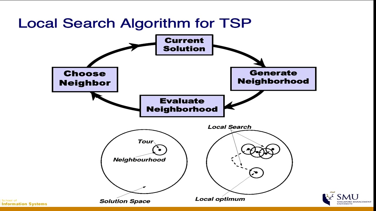
Local Search Algorithm for TSP — This diagram illustrates the core components of a local search algorithm. We start with a solution, generate its "neighborhood" of similar solutions, evaluate them, and move to a better one. This cycle repeats until no further improvement is possible.

A local search procedure is defined by a few key components:

An initial solution: This is our starting point. An excellent choice is to use a solution generated by a strong constructive heuristic like NEH.
A neighborhood structure: This defines the set of "neighboring" solutions that are reachable from the current solution by a single "move" or "operator".
A search strategy: This dictates how we explore the neighborhood and which neighbor we select to move to (e.g., the very first one that's better, or the absolute best one).
A stopping criterion: The search stops when we can't find any better neighbors, meaning we have reached a local optimum.

Defining the Neighborhood: The Swap Operator

For the permutation flow shop problem, a solution is a sequence of jobs ( $π$ ). A "move" is an operator that makes a small change to this sequence. One of the simplest and most common moves is the swap operator.

A swap simply involves exchanging the positions of two jobs in the sequence. For a sequence $π = (J_{1}, J_{2}, J_{3}, J_{4})$ , swapping the jobs at position 2 ( $J_{2}$ ) and position 4 ( $J_{4}$ ) would create the new sequence $π^{'} = (J_{1}, J_{4}, J_{3}, J_{2})$ .

The set of all possible solutions that can be generated by applying a single swap to the current solution forms its swap neighborhood. For a problem with $n$ jobs, there are $n (n - 1) /2$ possible pairs of jobs to swap, so the size of the neighborhood is $(2 n)$ .

Neighborhood Search Operators for Scheduling — This image shows three common operators. We are focusing on (a) the Swap operator, where two jobs exchange positions. The other operators, 'Insert', are also widely used and define a different neighborhood structure.

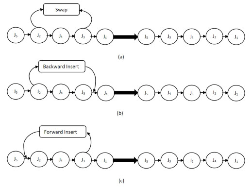
You might wonder why a simple swap is a good choice. For permutation scheduling, the relative order of jobs is critical. The swap operator is effective because it creates a new sequence that is still very similar to the old one, preserving much of the original relative ordering.

Introduction to Metaheuristics (8/9). Local search applied to the Travelling Salesman Problem

This video segment explains why certain operators are more suitable for permutation problems than others. The speaker highlights the importance of preserving relative order, which is exactly what the swap operator does.

Watch from 00:12:15 to 00:13:30. The key takeaway is that for permutation scheduling problems, the swap and insertion operators are appropriate because they maintain much of the existing job order, which is a desirable property for exploring the solution space effectively.

The Swap-Based Local Search Procedure

Now that we have the components, let's assemble the full procedure. The algorithm iteratively searches for improvements. In each iteration, it explores the neighborhood of the current best solution ( $π$ ) and, if a better solution is found, it updates $π$ and starts again.

There are two main strategies for choosing which neighbor to move to:

Best Improvement (or Steepest Descent): Evaluate all neighbors in the swap neighborhood. Select the neighbor that provides the largest improvement (i.e., the greatest reduction in makespan) and make that your new current solution. This is thorough but can be computationally expensive as you must evaluate every neighbor.
First Improvement: Evaluate the neighbors one by one. The moment you find a neighbor that is better than your current solution, you immediately move to it and start the next iteration from there. This is typically faster as you don't need to evaluate the entire neighborhood.

The process stops when a full search of the neighborhood yields no solution with a better makespan. At this point, the current solution is a local optimum with respect to the swap neighborhood.

The following resource provides a formal pseudo-code for a swap-based local search.

Enhanced Iterated Local Search Algorithms for the Permutation Flow Shop Problem...

The paper 'Enhanced Iterated Local Search Algorithms...' describes several components of advanced heuristics. We will focus on the clear and concise pseudo-code it provides for the basic swap-based local search.

Please read the section '3.2 Local Search Procedure', focusing on the description of the swap local search. Then, carefully study 'Figure 3: Pseudo code of the swap local search'. This figure formalizes the iterative procedure we've been discussing.

The pseudocode in Figure 3 outlines a systematic local search. It iterates through the jobs (idx) and considers swapping each one with jobs earlier in the sequence (line 7). If any swap leads to an improvement (line 8), the solution is updated, and a counter is reset to continue the search from the new, better solution. If a full pass over all jobs finds no improvement (cnt reaches n), the algorithm terminates, having found a local optimum.

Test your understanding!

In the previous lesson's exercise, you used the NEH heuristic on the following problem and found the sequence J1-J2-J3 with a makespan of 19.

Job	Machine 1	Machine 2	Machine 3
J1	5	2	6
J2	3	4	4
J3	4	3	2

Starting with the sequence $π = (J 1, J 2, J 3)$ , perform one iteration of a Best Improvement local search using the swap neighborhood.

List all unique neighbors of the sequence (J1, J2, J3) that can be created with a single swap.
Calculate the makespan for each neighbor.
Which sequence will be the new current solution after this iteration? What is its makespan?

Show answer

The initial sequence is $π = (J 1, J 2, J 3)$ with $C_{ma x} = 19$ .

1. Generate Swap Neighbors:
There are $(2 3) = 3$ possible swaps:

Swap J1 and J2: $π_{1} = (J 2, J 1, J 3)$
Swap J1 and J3: $π_{2} = (J 3, J 2, J 1)$
Swap J2 and J3: $π_{3} = (J 1, J 3, J 2)$

2. Calculate Makespan for Each Neighbor:

For $π_{1} = (J 2, J 1, J 3)$ :
- J2: M1(0-3), M2(3-7), M3(7-11)
- J1: M1(3-8), M2(8-10), M3(11-17)
- J3: M1(8-12), M2(12-15), M3(17-19)
- $C_{ma x} (π_{1}) = 19$
For $π_{2} = (J 3, J 2, J 1)$ :
- J3: M1(0-4), M2(4-7), M3(7-9)
- J2: M1(4-7), M2(7-11), M3(11-15)
- J1: M1(7-12), M2(12-14), M3(15-21)
- $C_{ma x} (π_{2}) = 21$
For $π_{3} = (J 1, J 3, J 2)$ :
- J1: M1(0-5), M2(5-7), M3(7-13)
- J3: M1(5-9), M2(9-12), M3(13-15)
- J2: M1(9-12), M2(12-16), M3(16-20)
- $C_{ma x} (π_{3}) = 20$

3. Select the Best Neighbor:
We compare the makespans of the neighbors to the current makespan of 19:

$C_{ma x} (π_{1}) = 19$ (No improvement)
$C_{ma x} (π_{2}) = 21$ (Worse)
$C_{ma x} (π_{3}) = 20$ (Worse)

Since none of the neighbors have a makespan better than 19, the sequence $π = (J 1, J 2, J 3)$ is already a local optimum for the swap neighborhood. The search terminates, and the solution remains (J1, J2, J3) with a makespan of 19. This demonstrates that even a good initial solution from NEH might already be locally optimal.

Conclusion

Today, we took the crucial step from constructing solutions to improving them. By understanding local search, you've unlocked the door to a vast and powerful set of optimization techniques that are central to modern scheduling research.

Key Takeaways:

Improvement heuristics, like local search, start with a complete solution and iteratively try to make it better. This contrasts with constructive heuristics, like NEH, which build a solution from scratch.
Local search operates by exploring a neighborhood of solutions, which are "close" to the current solution.
The swap operator is a simple and effective way to define a neighborhood for permutation scheduling problems. It involves exchanging the positions of any two jobs.
The local search procedure continues until it reaches a local optimum—a solution that is better than all of its immediate neighbors.
A powerful and common strategy is to use a constructive heuristic (NEH) to find a high-quality initial solution and then use local search to refine it.

Preview of the Next Lesson:
So far in this module, we've focused on heuristics that find good, but not necessarily optimal, solutions. How would we go about finding a provably optimal solution? In the next lesson, we will pivot from heuristics to exact optimization methods. You will learn how to formulate the permutation flow shop problem as a Mixed-Integer Linear Program (MILP). This will give you a new perspective on the problem structure and provide a foundation for understanding the trade-offs between heuristic and exact methods, a critical consideration for your thesis work.

Recommended resources

From Construction to Improvement: The Logic of Local Search

Defining the Neighborhood: The Swap Operator

The Swap-Based Local Search Procedure

Conclusion