Hello! Welcome to your next lesson on scheduling heuristics.
In our last session, we established a critical fact: the flow shop scheduling problem with three or more machines to minimize makespan ( for ) is NP-hard. This means that finding a guaranteed optimal solution becomes computationally intractable as the problem size grows. This is the fundamental reason why, for your thesis and in practical industrial applications, we turn to heuristics—intelligent methods that find high-quality, near-optimal solutions in a reasonable amount of time.
Today's lesson directly addresses this challenge by focusing on one of the most effective and widely-used heuristics for this problem. Our learning outcome is to apply the NEH heuristic to construct high-quality flow shop schedules.
We will cover:
- The core principle and steps of the NEH algorithm.
- A detailed, step-by-step application of the heuristic to a sample problem.
- The distinction between constructive heuristics like NEH, which build a solution from scratch, and improvement heuristics, which we will discuss in the next lesson.
The NEH Heuristic: A Powerful Constructive Method
The NEH heuristic, named after its creators Nawaz, Enscore, and Ham, is a constructive heuristic. Its main goal is to build a single, high-quality sequence from the ground up.
The intuition behind NEH is both simple and powerful: jobs that require a large amount of total processing time across all machines are likely to be more "critical" and should be scheduled with priority. By placing these high-workload jobs earlier in the sequencing process, the algorithm has more flexibility to fit the smaller jobs around them, aiming to reduce idle time and, consequently, the overall makespan ().
The algorithm consists of two main phases:
- Initial Job Ordering: An initial sequence of jobs is created not for scheduling, but as a priority list. This list is formed by sorting the jobs in descending order of their total processing times summed across all machines.
- Iterative Insertion: The final schedule is built incrementally. The algorithm takes the first job from the priority list, then the second, and finds the best sequence for just those two. It then takes the third job and inserts it into the best possible position within the existing two-job sequence. This "insert and evaluate" process continues until all jobs from the priority list have been placed.
Let's look at a more formal description.
A new constructive heuristic for the No-Wait Flowshop ...
The following resource provides a concise, formal description of the NEH algorithm. It's a clear summary of the two steps we just discussed.
Please read the paragraph that begins 'The principle of NEH heuristic is...' and review 'Algorithm 1: NEH'. This will solidify your understanding of the procedure before we see it in action.
Applying the NEH Algorithm: A Worked Example
The best way to understand an algorithm is to see it in action. The following video provides an excellent, step-by-step walkthrough of the NEH heuristic applied to a 5-job, 3-machine problem. It clearly demonstrates the iterative insertion process and the makespan calculations at each step.
Mod-07 Lec-27 Flow shop scheduling -- heuristics -- Palmer, Campbell Dudek Smith algorithm
This video segment, from a lecture by Prof. G. Srinivasan of IIT Madras, demonstrates the NEH algorithm. Pay close attention to how the partial sequences are built and how the makespan is calculated for each possible insertion to decide which sequence to keep.
Watch the segment from 00:46:44 to 00:54:42. The presenter first calculates the total processing times to get the initial priority order. Then, he iteratively builds the schedule by inserting jobs and selecting the partial sequence with the minimum makespan.
As you saw in the video, the NEH algorithm methodically explores the most promising sequences based on its core principle. The final sequence it produced, (J3, J4, J5, J1, J2), resulted in a makespan of 106. This was better than the solutions found by two other common heuristics (Palmer's and CDS) for that specific problem instance.
To reinforce this process, you can also review another worked example in the thesis "Permutation Flow Shop via Simulated Annealing and NEH". This document walks through a 5-job, 4-machine problem with helpful Gantt charts visualizing the makespan at each step. You can find this example in Section 4.1.1 of the resource with resource ID LINK.
Visualizing the Goal
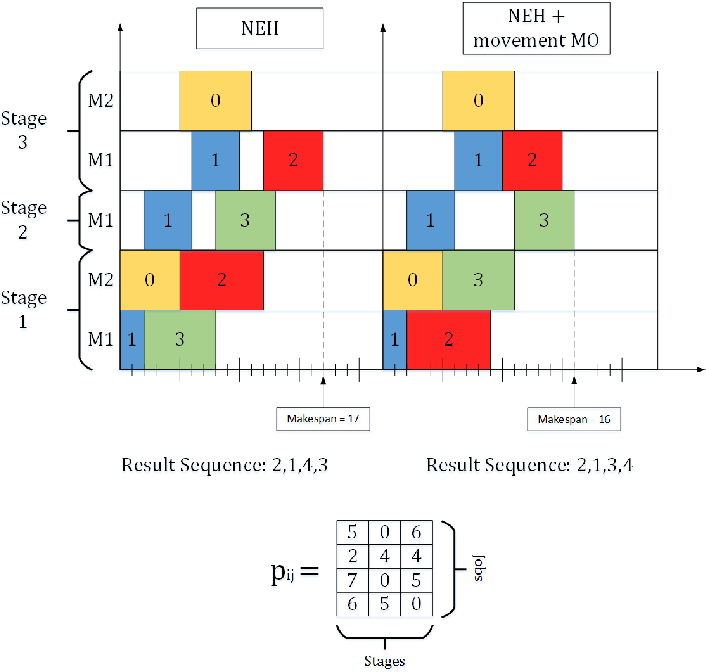
The entire purpose of heuristics like NEH is to arrange the blocks on a Gantt chart in a way that the final completion time is minimized. A good heuristic creates a schedule that is "densely packed," minimizing the idle time on machines.

Different sequences yield different makespans. The NEH heuristic is designed to find a sequence that produces a makespan that is optimal or very close to optimal, as shown in the comparison below where the NEH-based method finds a sequence with a makespan of 16, while another method results in 17.
Test your understanding!
Let's apply the NEH algorithm yourself. Consider the following 3-job, 3-machine flow shop problem. Your task is to find the best sequence and the corresponding makespan using the NEH heuristic.
| Job | Machine 1 | Machine 2 | Machine 3 |
|---|---|---|---|
| J1 | 5 | 2 | 6 |
| J2 | 3 | 4 | 4 |
| J3 | 4 | 3 | 2 |
Follow the NEH steps:
- Calculate the total processing time for each job and create the initial priority list.
- Take the first two jobs from the list and find the better of the two possible sequences.
- Insert the third job into all possible positions in the sequence from step 2 and find the best final sequence.
- Calculate the makespan for the final sequence.
Show answer
Step 1: Initial Job Ordering
- Total time for J1:
- Total time for J2:
- Total time for J3:
Sorting in descending order of total time gives the priority list: (J1, J2, J3).
Step 2: Sequence the first two jobs (J1, J2)
We evaluate two partial sequences: J1-J2 and J2-J1.
-
Sequence J1-J2:
- J1: M1(0-5), M2(5-7), M3(7-13)
- J2: M1(5-8), M2(8-12), M3(13-17)
- Makespan = 17
-
Sequence J2-J1:
- J2: M1(0-3), M2(3-7), M3(7-11)
- J1: M1(3-8), M2(8-10), M3(11-17)
- Makespan = 17
Both sequences yield the same makespan. Let's arbitrarily choose J1-J2 as our current best sequence.
Step 3: Insert the third job (J3)
We insert J3 into all possible positions of the sequence J1-J2:
- J3-J1-J2
- J1-J3-J2
- J1-J2-J3
-
Sequence J3-J1-J2 (Makespan = 22):
- J3: M1(0-4), M2(4-7), M3(7-9)
- J1: M1(4-9), M2(9-11), M3(11-17)
- J2: M1(9-12), M2(12-16), M3(17-21) -> Mistake in calculation here. Let's re-calculate.
- J2 on M1: starts at 9, ends at 12.
- J2 on M2: starts at
max(12, 11)=12, ends at 16. - J2 on M3: starts at
max(16, 17)=17, ends at 21. Makespan is 21.
-
Sequence J1-J3-J2 (Makespan = 19):
- J1: M1(0-5), M2(5-7), M3(7-13)
- J3: M1(5-9), M2(9-12), M3(13-15)
- J2: M1(9-12), M2(12-16), M3(16-20) -> Re-calculate.
- J2 on M1: starts at 9, ends at 12.
- J2 on M2: starts at
max(12, 12)=12, ends at 16. - J2 on M3: starts at
max(16, 15)=16, ends at 20. Makespan is 20.
-
Sequence J1-J2-J3 (Makespan = 19):
- J1: M1(0-5), M2(5-7), M3(7-13)
- J2: M1(5-8), M2(8-12), M3(13-17)
- J3: M1(8-12), M2(12-15), M3(17-19)
- Makespan is 19.
Comparing the makespans (21, 20, 19), the minimum is 19.
Step 4: Final Result
The best sequence found is J1-J2-J3 with a makespan of 19.
Conclusion
In this lesson, we moved from theory to practice. Acknowledging the NP-hardness of the flow shop problem, we learned how to apply the NEH heuristic to construct a high-quality schedule efficiently.
Key Takeaways:
- The NEH heuristic is a constructive method for the permutation flow shop problem with makespan minimization.
- Its guiding principle is to prioritize jobs with higher total processing times.
- The algorithm works in two stages: an initial sort to create a priority list, followed by an iterative insertion process where jobs are added one by one into the position that yields the best partial makespan.
- NEH is widely regarded as one of the best-performing constructive heuristics for this problem, providing an excellent balance between solution quality and computational speed.
Preview of the Next Lesson:
We have now learned how to build a good solution from nothing. But what if we want to make it even better? In the next lesson, we will explore improvement heuristics. You will learn how to implement a swap-based local search procedure that can take an existing schedule (like one generated by NEH) and try to improve it by making small, systematic changes. This will be our first step into the broader field of local search and metaheuristics, which are central to your thesis topic.