Permutation Flow Shop MILP Model

From Shop Floor Rules to Mathematical Equations

The challenge of mathematical modeling is to translate the physical rules and objectives of a system into the language of mathematics. For the permutation flow shop problem (PFSP) with a makespan ($C_{max}$) objective, we have the following rules:

• All jobs follow the same machine sequence: M1 → M2 → ... → Mm.
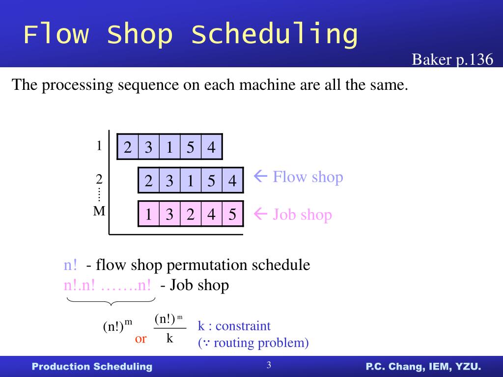
• The job sequence is the same on all machines (this is the "permutation" aspect).
• A machine can only process one job at a time.
• A job cannot be processed on machine i+1 until it has finished on machine i.
• The goal is to find the job sequence that minimizes the time the last job finishes on the last machine.

With $n$ jobs, there are $n!$ possible sequences. For even a modest 10 jobs, this is over 3.6 million possibilities! A MILP allows us to represent all these possibilities within a single model and have a solver efficiently search for the best one.

Formulation 1: The Position-Based Model

One of the most intuitive ways to model a permutation is to create decision variables that assign each job to a specific position in the sequence. Let's say we have positions $k=1,2,...,n$. Our model will decide which job goes into which position.

We will study a well-known formulation by Stafford et al. It's clean, effective, and provides a great introduction to the topic.

To start, let's define our terms:

• Indices:
  • $i\in \{1,...,m\}$ for machines.
  • $j\in \{1,...,n\}$ for jobs.
  • $k\in \{1,...,n\}$ for positions in the sequence.
• Parameter:
  • $p_{ij}$: Processing time of job $j$ on machine $i$.

Now, let's look at the full formulation.

Let's break down this model.

Decision Variables

The model uses two types of variables:

1. $x_{jk}\in \{0,1\}$: A binary variable. It equals 1 if job $j$ is assigned to position $k$ in the sequence, and 0 otherwise. This is the core of our sequence decision.
2. $f_{ik}\ge 0$: A continuous variable representing the finish time of the job in position $k$ on machine $i$.

Objective Function

$\min f_{mn}$

This is simple and elegant. We want to minimize the finish time of the job in the last position ($k=n$) on the last machine ($i=m$). By definition, this is the makespan ($C_{max}$).

Constraints

1. Assignment Constraints:
   ${\sum }_{k=1}^n{x}_{jk}=1(\forall j=1,...,n)$
   ${\sum }_{j=1}^n{x}_{jk}=1(\forall k=1,...,n)$
   These two sets of equations ensure a valid one-to-one assignment. The first says that every job must be assigned to exactly one position. The second says that every position must be filled by exactly one job.

2. Finish Time Calculation:
   The magic of the model lies in how it calculates finish times. The term ${\sum }_{j=1}^n{p}_{ij}{x}_{jk}$ cleverly picks out the processing time of whichever job $j$ is assigned to position $k$. Since only one $x_{jk}$ will be 1 for a given $k$, this sum equals exactly the processing time of the job in position $k$ on machine $i$.

   • First job, first machine:
     $f_{11}={\sum }_{j=1}^n{p}_{1j}{x}_{j1}$
     The finish time of the first job in the sequence on the first machine is simply its processing time.

   • Machine precedence (Job in position k on machine i):
     $f_{i+1,k}\ge f_{ik}+{\sum }_{j=1}^n{p}_{i+1,j}{x}_{jk}(\forall i,k)$
     This enforces the flow shop routing. The finish time of a job on machine $i+1$ must be greater than or equal to its finish time on machine $i$ plus its processing time on machine $i+1$.

   • Sequence precedence (Machine i processing job in position k):
     $f_{i,k+1}\ge f_{ik}+{\sum }_{j=1}^n{p}_{ij}{x}_{j,k+1}(\forall i,k)$
     This ensures that on any machine $i$, the job in position $k+1$ cannot start until the job in position $k$ is finished.

The use of $\ge$ instead of $=$ is important. It allows for idle time on machines or waiting time for jobs, which is necessary to maintain feasibility. Since we are minimizing $f_{mn}$, the solver will naturally push all finish times to be as early as possible.

Formulation 2: The Precedence-Based Model

An alternative approach is to define variables based on the relative order of jobs, rather than their absolute position. This type of model is often based on the work of Manne.

The key decision variable is:

• $z_{ij}\in \{0,1\}$: Equals 1 if job $i$ precedes job $j$ (not necessarily immediately), and 0 if job $j$ precedes job $i$. We only need to define this for $i<j$ to avoid redundancy.

The other main variable tracks completion times by job, not by position:

• $C_{ik}\ge 0$: A continuous variable representing the completion time of job $i$ on machine $k$.

This paper on MILP models presents several formulations. We will focus on the one called MUB3, which is based on Manne's model. Note that the paper's objective is to minimize earliness and tardiness, but we can easily adapt its core constraints for our makespan objective.

Let's adapt the MUB3 model for a makespan objective.

Objective Function

$\min C_{max}$
subject to:
$C_{max}\ge C_{im}(\forall i=1,...,n)$
We introduce a new variable, $C_{max}$, and add constraints that force it to be greater than or equal to the completion time of every job on the final machine. Minimizing $C_{max}$ achieves our goal.

Constraints

1. Job Precedence (within a job):
   $C_{ik}\ge C_{i,k-1}+p_{ik}(\forall i,k>1)$
   This is the same logic as before: a job's completion on machine $k$ depends on its completion on machine $k-1$.

2. Machine Precedence (between jobs): This is where the model is fundamentally different.
   $C_{jk}\ge C_{ik}+p_{jk}-M(1-z_{ij})(\forall k,i<j)$
   $C_{ik}\ge C_{jk}+p_{ik}-M{z}_{ij}(\forall k,i<j)$
   These are called disjunctive constraints. They ensure that on any machine $k$, only one job is processed at a time. Let's see how they work for any pair of jobs $i$ and $j$:

   • Case 1: Job $i$ precedes job $j$. Then $z_{ij}=1$.
     • The first constraint becomes $C_{jk}\ge C_{ik}+p_{jk}$. This is active and enforces that job $j$ cannot complete before job $i$ is complete plus its own processing time.
     • The second constraint becomes $C_{ik}\ge C_{jk}+p_{ik}-M$. Since M is a very large number, this constraint becomes $C_{ik}\ge (\text{something})-M$, which is always true and thus inactive.
   • Case 2: Job $j$ precedes job $i$. Then $z_{ij}=0$.
     • The first constraint becomes $C_{jk}\ge C_{ik}+p_{jk}-M$. This is inactive.
     • The second constraint becomes $C_{ik}\ge C_{jk}+p_{ik}$. This is active and enforces the correct sequence.

This "big-M" technique is a standard and powerful tool in MILP for modeling logical choices.

Comparing the Formulations

We have seen two ways to model the same problem:

1. Position-based: Uses variables $x_{jk}$ to assign jobs to positions. It is often more intuitive for permutation problems.
2. Precedence-based: Uses variables $z_{ij}$ to define the relative order of job pairs. It can be more generalizable to non-permutation problems like the job shop.

These models differ in size (number of variables and constraints), which affects how quickly a solver can find the optimal solution. For your thesis, being able to choose or design the right formulation for a specific problem variant is a key skill. The precedence-based formulation, for example, is a more natural starting point when modeling the general job shop problem, which you will encounter later.

Conclusion

Today we moved from the world of heuristics to the world of exact optimization by modeling the permutation flow shop as a Mixed-Integer Linear Program. You now have a powerful tool to find provably optimal solutions, providing a vital baseline for your research.

Key Takeaways:

• MILP is a method for finding optimal solutions to problems by defining an objective, decision variables, and constraints mathematically.
• Position-based formulations use binary variables to assign jobs to positions in a sequence (e.g., $x_{jk}$).
• Precedence-based formulations use binary variables to define the relative order between any pair of jobs (e.g., $z_{ij}$).
• The "big-M" method is a common technique in MILP to model disjunctive "either-or" constraints, which are essential for preventing two jobs from occupying the same machine at the same time.

Preview of the Next Lesson:
We have now explored two distinct approaches to the flow shop problem: fast heuristics that find good solutions (NEH, local search) and exact methods that find optimal solutions but can be slow (MILP). In our next lesson, we will step back to compare constructive vs. improvement heuristics. This will consolidate your understanding of heuristic design and set the stage for later modules where you'll learn about advanced metaheuristics that try to combine the speed of heuristics with the quality-seeking power of more exhaustive methods.