Hello! Welcome to your next lesson on solving the Flexible Job Shop Problem (FJSP).
In our last session, we constructed a complete Mixed-Integer Linear Program (MILP) for the FJSP. That integrated model is powerful because it captures all assignment and sequencing decisions simultaneously, guaranteeing an optimal solution if solved to completion. However, as you know from your engineering background, the computational effort required to solve such NP-hard problems to optimality grows explosively with problem size. For your thesis work on real-world scale problems, relying solely on an integrated MILP will be impractical.
This brings us to today's topic: a fundamentally different strategy. Our goal is to apply hierarchical approaches to solve the FJSP. Instead of tackling the problem all at once, we will "divide and conquer" by breaking it down into more manageable subproblems. This lesson is a crucial bridge between the exact, integrated models we've studied and the practical heuristics and metaheuristics you'll need for your research.
The "Divide and Conquer" Strategy: Hierarchical Approaches
The core idea behind hierarchical approaches is to decompose the FJSP into its two fundamental components and solve them sequentially. This strategy trades the guarantee of optimality for significant gains in computational speed and scalability.
To begin, let's get a formal definition of this method.
Solving Flexible Job Shop Scheduling with Multi Objective ...
The paper 'Solving Flexible Job Shop Scheduling with Multi Objective...' provides a concise introduction to hierarchical versus integrated approaches. It gives historical context and clearly defines the decomposition.
Please read the introduction section of the paper. Focus on the paragraph that begins 'For solving the realistic case...'. Pay attention to how it defines hierarchical and integrated approaches and the reference to Brandimarte's seminal work, which first applied this decomposition.
As the paper highlights, the hierarchical method splits the FJSP into two distinct stages:
- Stage 1: The Machine Assignment Subproblem (Routing). In this stage, we decide which machine will perform each operation. We essentially fix the routing for every job, ignoring the detailed sequencing of operations for the moment.
- Stage 2: The Operation Sequencing Subproblem (Scheduling). With the machine assignments now fixed from Stage 1, the problem is simplified. It becomes a standard Job Shop Scheduling Problem (JSP), where the task is to sequence the operations assigned to each machine to minimize the objective (e.g., makespan).
This separation of concerns is a classic engineering strategy for managing complex systems.
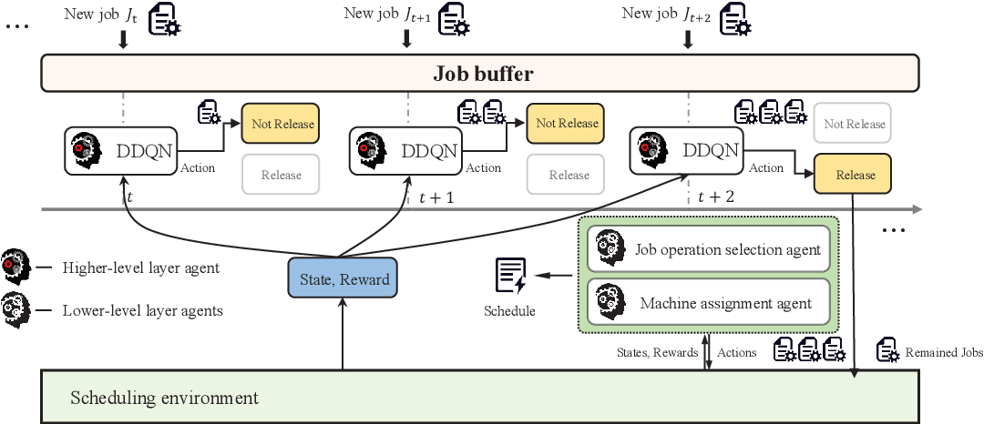
The primary drawback of this method is that the decisions made in Stage 1 are irrevocable and might not lead to the globally optimal solution. An assignment that looks good in isolation (e.g., assigning an operation to its fastest machine) might create an unavoidable bottleneck in Stage 2. A truly optimal schedule might require a "bad" assignment locally to achieve a better overall result.
Stage 1: Solving the Assignment Problem
The first task is to assign every operation to a machine from its set of eligible machines . The goal is to make "good" assignments that will likely lead to a good final schedule. Here are a few common heuristics for this stage:
- Shortest Processing Time (SPT) Assignment: Assign each operation to the machine that can process it the fastest. This is a greedy, intuitive rule that aims to minimize the total time spent in processing.
- Workload Balancing Assignment: Assign the next operation to the eligible machine that currently has the minimum total processing time of all operations already assigned to it. This heuristic tries to distribute the work evenly to avoid creating a single, heavily loaded bottleneck machine.
- Random Assignment: Assign each operation to a random eligible machine. While seemingly naive, this can be a useful baseline or a starting point for more advanced improvement algorithms.
Let's consider the physical system we're modeling.

Stage 2: Solving the Sequencing Problem
Once Stage 1 is complete, we have a fixed set of operations assigned to each machine. The problem is no longer an FJSP; it has been reduced to a classical Job Shop Scheduling Problem (JSP). Now, we must determine the sequence of operations on each machine.
You have already encountered methods for this in previous lessons:
- Dispatching Rules: We can apply rules locally on each machine to decide which of its waiting jobs to process next. Examples include First-In-First-Out (FIFO), Shortest Processing Time (SPT), or Earliest Due Date (EDD).
- Constructive Heuristics for JSP: The Giffler-Thompson algorithm, which we covered in Module 5, is designed specifically for this. It can be applied directly to the problem resulting from Stage 1 to generate a feasible and active schedule.
- Improvement Heuristics: One could start with a simple sequence (e.g., from a dispatching rule) and then apply a local search procedure, like the swap-based methods from the flow shop module, to improve the makespan. Brandimarte's original paper used a Tabu Search metaheuristic in this stage.
A Walkthrough Example
Let's make this concrete with a small example.
Problem Instance:
- Job 1:
- Job 2:
- Processing Times :
| Operation | Machine M1 | Machine M2 | Machine M3 |
|---|---|---|---|
| 5 | 8 | - | |
| - | 6 | 7 | |
| 9 | - | 11 | |
| 10 | 4 | - |
Step 1: Hierarchical Approach - Stage 1 (Assignment)
Let's use the SPT assignment rule.
- For : M1 (p=5) is faster than M2 (p=8). Assign to M1.
- For : M2 (p=6) is faster than M3 (p=7). Assign to M2.
- For : M1 (p=9) is faster than M3 (p=11). Assign to M1.
- For : M2 (p=4) is faster than M1 (p=10). Assign to M2.
Result of Stage 1: The assignments are now fixed.
- M1 processes: (p=5) and (p=9).
- M2 processes: (p=6) and (p=4).
- M3 processes: Nothing.
Step 2: Hierarchical Approach - Stage 2 (Sequencing)
We now have a standard JSP. We need to sequence the operations on M1 and M2.
- On M1: Sequence (, ) or (, )?
- On M2: Sequence (, ) or (, )?
Let's apply a simple sequencing rule: process operations in the order of their job index, then operation index.
- On M1: comes before . Sequence is .
- On M2: comes before . Sequence is .
Now we can build the schedule (e.g., by drawing a Gantt chart):
- At t=0, starts on M1. It finishes at t=5.
- At t=0, could potentially start on M2, but it must wait for . So M2 is idle.
- At t=5, finishes. M1 is now free. can start. It runs from t=5 to t=14.
- Also at t=5, finishing means can start on M2. It runs from t=5 to t=11.
- At t=11, finishes on M2.
- At t=14, finishes on M1. Now can start on M2. M2 is free since t=11. So starts on M2 at t=14. It runs from t=14 to t=18.
The last operation to finish is at t=18. The makespan is 18.
Test your understanding!
Let's re-run the example. Suppose in Stage 1, we used a different rule that resulted in the following assignments:
- is assigned to M2 (p=8).
- is assigned to M2 (p=6).
- is assigned to M1 (p=9).
- is assigned to M1 (p=10).
- What scheduling problem is created after these assignments are fixed? Describe which operations compete for which machines.
- Using the same sequencing rule ("by job index, then operation index"), what would be the makespan? Is it better or worse than the 18 we got with the SPT assignment?
Show answer
-
Resulting Problem: We have a JSP where M1 processes and M2 processes . This is actually simpler than a general JSP; it has decomposed into two independent 2-operation flow shops, one for each job on its assigned machines. Wait, the jobs are not on the same machines. Job 1 is on M2 and Job 2 is on M1. The problem decomposes into two independent single-machine sequencing problems with precedence constraints. M1 must sequence then . M2 must sequence then .
-
Makespan Calculation:
- On M2: runs from t=0 to t=8. Then runs from t=8 to t=14.
- On M1: runs from t=0 to t=9. Then runs from t=9 to t=19.
- The latest completion time is 19. The new makespan is 19. This is worse than the makespan of 18 from our first attempt. This demonstrates how the initial assignment decisions can significantly impact the final solution quality.
Conclusion
In this lesson, we explored a practical and widely-used strategy for tackling the complex FJSP: hierarchical decomposition. By separating the problem into assignment and sequencing stages, we can leverage simpler, faster heuristics to find good solutions for large problem instances where exact methods fail.
Key Takeaways:
- Hierarchical approaches solve the FJSP by decomposing it into two subproblems: machine assignment (routing) followed by operation sequencing (scheduling).
- This "divide and conquer" strategy drastically reduces computational complexity at the potential cost of solution optimality.
- Stage 1 (Assignment) can be solved using heuristics like Shortest Processing Time (SPT) or workload balancing.
- Stage 2 (Sequencing) solves the resulting Job Shop Problem, often using dispatching rules (e.g., FIFO) or dedicated JSP algorithms (e.g., Giffler-Thompson).
Preview of the Next Lesson:
Our simple hierarchical model made assignments based only on processing time. But as your thesis requires, real-world factories have additional complexities. What if changing from one job to another on a machine requires a lengthy setup? What if jobs need to be moved between work centers by a limited number of vehicles?
In the next module, we will begin tackling these challenges. Our first lesson will focus on distinguishing between sequence-independent and sequence-dependent setup times and how to start incorporating them into our models. This will add another layer of realism and complexity, moving us closer to the models you will develop in your research.