Hello! Welcome to your lesson on formulating the Flexible Job Shop Problem (FJSP) as a Mixed-Integer Linear Program (MILP).
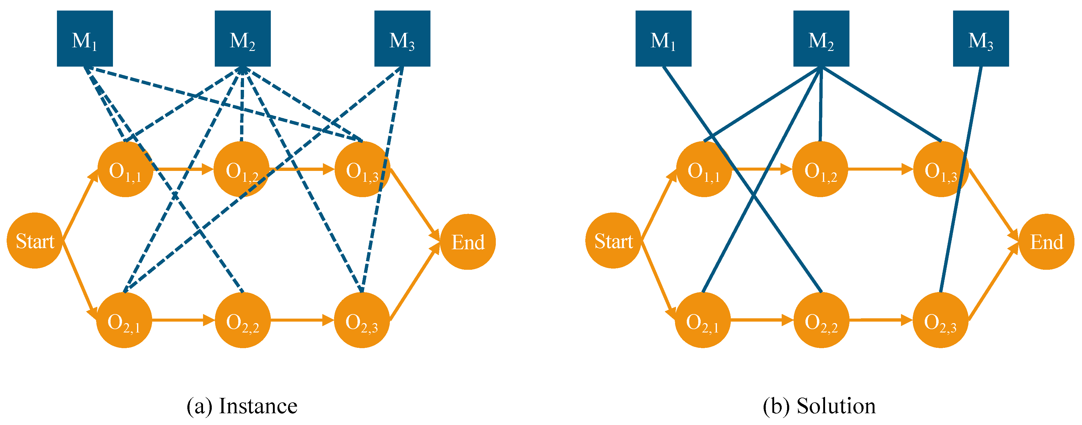
In our last session, we established that the FJSP can be conceptually decomposed into two subproblems: machine assignment (routing) and operation sequencing. We also touched on how this decomposition influences the design of solution methods, categorizing them as either hierarchical (solving in stages) or integrated (solving simultaneously).
Today, our goal is to translate that conceptual framework into a precise, mathematical language. We will formulate the FJSP as a MILP model, which is an integrated approach that solves both subproblems at once. For your thesis work, mastering MILP formulation is a cornerstone skill. It not only provides a method for finding optimal solutions for smaller problems but also serves as a formal problem definition and a benchmark against which you can compare the heuristics and metaheuristics you will develop later.
From Physical System to Mathematical Model
Before we dive into the equations, let's establish a clear framework for what a MILP model entails. We are essentially creating a mathematical representation of the physical job shop system.
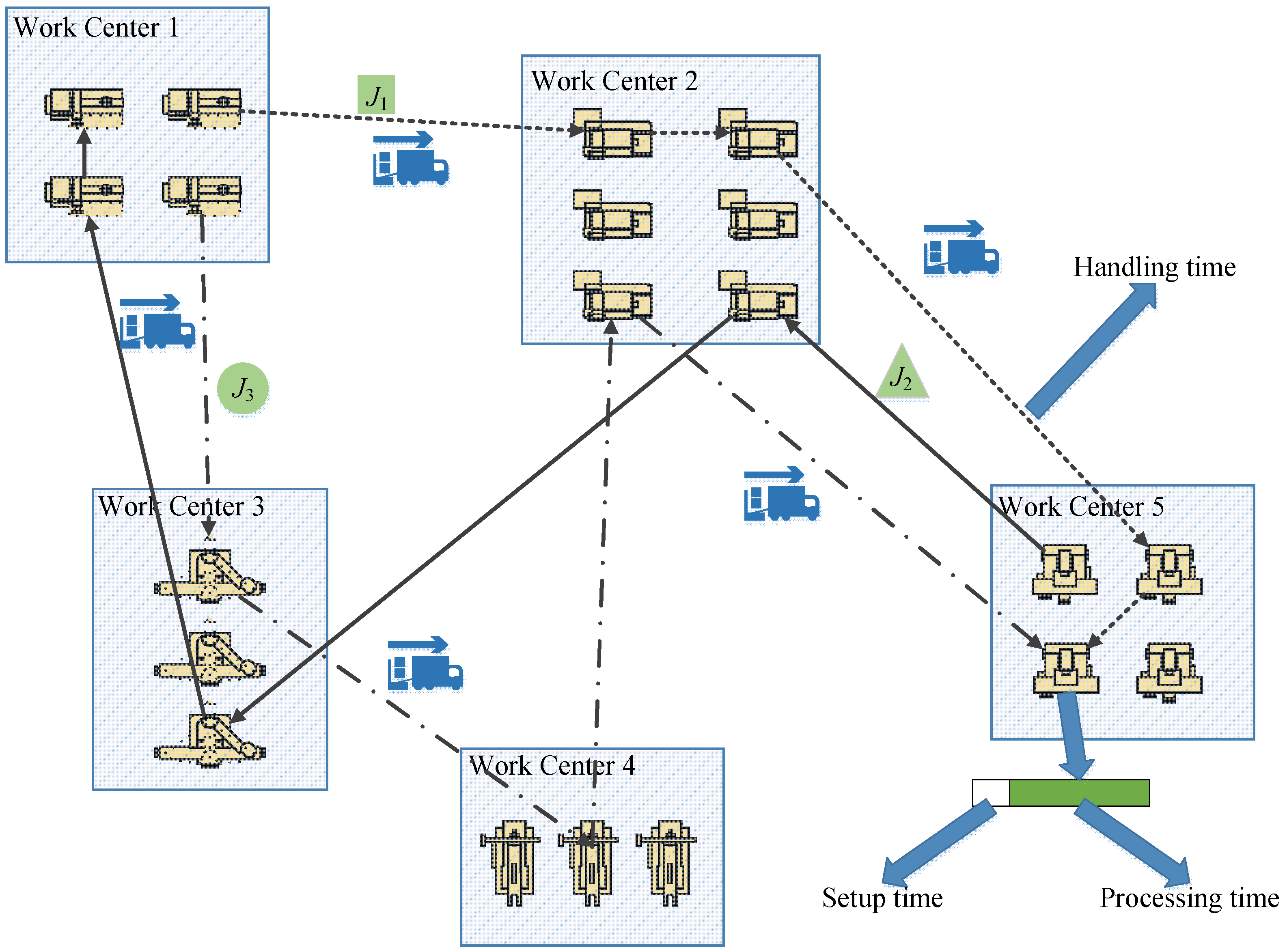
To build the model, we need four key ingredients:
- Indices and Sets: Symbols that represent the objects in our system (e.g., jobs, operations, machines).
- Parameters: The known data about the problem instance (e.g., the processing time of a specific operation on a specific machine).
- Decision Variables: The unknown values our model must determine. These represent the decisions we need to make—namely, machine assignments and operation sequences. They can be continuous (like a start time) or binary (representing a yes/no choice).
- Objective Function & Constraints: The goal we want to achieve (e.g., minimize makespan) and the rules that any valid schedule must follow (e.g., precedence relations, machine capacity).
With this structure in mind, we will now build a complete MILP formulation.
A Sequence-Based MILP Formulation for FJSP
There are many ways to formulate the FJSP. We will start with a classic and intuitive sequence-based approach that directly mirrors the assignment and sequencing decomposition we discussed previously. This type of model is often called a "disjunctive" formulation.
The following reading presents two MILP models. We will focus on the second one, which they call the "alternative model" or Alt-Cmax. It uses separate variables for the assignment and sequencing decisions, making it a clear example of a hierarchical representation within an integrated model.
An efficient algorithm for solving the flexible job shop ...
The paper 'An efficient algorithm for solving the flexible job shop...' by Thörnblad et al. provides a very clear sequence-based MILP formulation. We will use this as our primary reference.
Please read Section 3.1, 'Indices, sets, and parameters', to familiarize yourself with the notation. Then, carefully study Section 3.3, 'An alternative model'. Focus on understanding the decision variables and the purpose of each constraint from (3b) to (3j).
Let's break down the Alt-Cmax model from the paper step-by-step.
1. Indices, Sets, and Parameters
- Indices:
- : indices for jobs.
- : indices for operations. denotes the -th operation of job .
- : index for machines (or resources).
- Sets:
- : set of all jobs.
- : set of operations for job .
- : set of all machines.
- : set of eligible machines that can process operation .
- Parameters:
- : processing time of operation on machine .
- : a very large positive number (the "big-M").
2. Decision Variables
These variables directly capture the assignment and sequencing decisions:
- Assignment Variable (Routing):
- : A binary variable that is 1 if operation is assigned to machine , and 0 otherwise. This variable solves the routing subproblem.
- Sequencing Variable:
- : A binary variable that is 1 if operation precedes operation on machine , and 0 otherwise. This variable solves the sequencing subproblem for operations assigned to the same machine.
- Timing Variable:
- : A continuous variable representing the start time of operation on machine .
- Objective Variable:
- : A continuous variable representing the makespan (the completion time of the last job).
3. Objective Function
The goal is to minimize the makespan:
4. Constraints
These are the rules that enforce a valid schedule.
-
Assignment Constraint (Constraint 3b): Each operation must be assigned to exactly one of its eligible machines.
-
Precedence Constraints (Constraint 3f): An operation cannot start before its direct predecessor in the same job has finished. For operation followed by :
Note: The paper's formulation(3f)is slightly different but achieves the same goal. The version above is a common way to write it. -
Disjunctive Constraints (Constraints 3d, 3e): This is the core of the sequencing logic. For any two operations, and , that could potentially be processed on the same machine , one must finish before the other starts.
Let's analyze this pair of "big-M" constraints. The variable acts as a switch.- If , it means is scheduled before on machine .
- The first constraint becomes , ensuring starts after finishes.
- The second constraint becomes . Since M is huge, this constraint becomes redundant and non-binding.
- If , it means is scheduled before on machine . The logic is reversed.
These constraints only apply if both operations are actually assigned to machine (i.e., when and ).
- If , it means is scheduled before on machine .
-
Makespan Definition (Constraint 3g): The makespan must be greater than or equal to the completion time of every operation.
The combination of these variables, objective, and constraints forms a complete MILP model that an optimization solver (like Gurobi or CPLEX) can process to find an optimal schedule.
Test your understanding!
Consider a small FJSP instance:
- Job 1:
- Job 2:
Machine eligibility and processing times:
- : M1 (p=5), M2 (p=6)
- : M2 (p=4)
- : M1 (p=8)
Based on the MILP formulation we just studied, write out the following specific constraints for this instance:
- The assignment constraint for operation .
- The precedence constraint between and .
- The pair of disjunctive constraints for operations and on machine M1. (Assume is 1 if precedes on M1).
Show answer
-
Assignment constraint for :
Operation can be on M1 or M2. The constraint ensures it is assigned to exactly one. -
Precedence constraint for Job 1:
Operation must start after is complete. The start time of (which can only be on M2) must be greater than the completion time of (which could be on M1 or M2).
Since and are binary and sum to 1, exactly one of the terms in the parentheses will be non-zero in the final solution. -
Disjunctive constraints for and on M1:
These operations might compete for machine M1.- If ( before ):
- If ( before ):
Note: will always be 1 since has no other machine choice. These constraints enforce that if is also 1, the two operations cannot overlap on M1.
- If ( before ):
The Landscape of FJSP Formulations
The sequence-based model is just one of several ways to formulate the FJSP. For your thesis research, it's beneficial to be aware of the other main paradigms, as they have different characteristics in terms of model size and solver performance.
The thesis by Azadeh et al. that we looked at previously provides an excellent and deep survey of these alternatives.
Mathematical Modelling and Optimization of Flexible Job Shops ...
To broaden your understanding of different modeling approaches, I recommend reviewing the key MILP formulations presented in 'Mathematical Modelling and Optimization of Flexible Job Shops...'.
You don't need to read this in full detail right now, but please skim Section 3.4 ('Enhanced position-based MILP (MILP-2)') and the start of Section 3.5 ('Sequence-based MILPs'). Notice the fundamental difference in the main binary variable: Position-based (MILP-2): The variable assigns an operation to a specific position or slot on a machine. This is an integrated variable. Sequence-based (MILP-4, MILP-5): These use separate variables for assignment and sequencing, similar to the model we just studied.
The key takeaway is that different choices of decision variables lead to fundamentally different model structures.
- Sequence-based models (like the
Alt-Cmaxwe detailed) are generally more intuitive but can have a very large number of sequencing variables (). - Position-based models create a "slot" for each potential operation on a machine's schedule. They can be more compact but sometimes yield weaker linear relaxations, making them slower for a solver to prove optimality.
Knowing these alternatives will be invaluable when you review literature for your thesis or decide on a baseline model for your own work.
Conclusion
In this lesson, we have taken the conceptual idea of the FJSP and translated it into a formal, solvable Mixed-Integer Linear Program. This is a critical step from understanding a problem to optimizing it.
Key Takeaways:
- An FJSP can be formulated as a MILP using indices, parameters, decision variables, an objective function, and constraints.
- The core of the formulation involves binary assignment variables (like ) to handle the routing subproblem and binary sequencing variables (like ) to handle the sequencing subproblem.
- "Big-M" constraints are a standard and powerful technique for modeling the "either-or" logic required to prevent operations from overlapping on a machine.
- The sequence-based formulation we studied is just one approach; other paradigms like position-based models also exist and offer different trade-offs.
Preview of the Next Lesson:
While the integrated MILP model we built is powerful, it can be very difficult to solve for large, real-world problems. This motivates other approaches. In our next lesson, we will explore hierarchical approaches to solve the FJSP. Instead of solving everything at once, these methods first solve the assignment problem and then solve the sequencing problem in a second step. This will provide a practical contrast to the MILP model and serve as a bridge to understanding more advanced heuristic methods.