Sequence-Dependent vs. Sequence-Independent Setup Times

Hello! Welcome to the next phase of our course.

In our last lesson, we explored hierarchical approaches for solving the Flexible Job Shop Problem (FJSP), breaking it down into more manageable assignment and sequencing subproblems. We noted that this approach, while practical, relies on simplified models. Your thesis, however, requires tackling the complexities of real-world manufacturing, such as the time lost when preparing a machine for its next task.

This lesson marks our entry into Module 7, where we begin to model these complex constraints. Our learning outcome today is to distinguish between sequence-independent and sequence-dependent setup times. This foundational concept is the first and most critical step before we can incorporate these constraints into the advanced optimization models you'll need for your research.

What is a Setup Time?

In any production environment, a "setup" refers to the activities required to prepare a machine or resource to process a job. As an industrial engineer, you're likely familiar with this. Setups can include:

Changing tools on a CNC machine.
Cleaning a vessel in a chemical plant between different product batches.
Calibrating measurement equipment.
Loading a specific mold into an injection-molding machine.

In many introductory scheduling models, setup time is either ignored or simply included as part of the job's processing time. However, in many real-world systems, especially those with high product variety, explicitly modeling setup times is essential for creating efficient and realistic schedules.

The Fundamental Distinction: Sequence-Independent vs. Sequence-Dependent

The key to modeling setups correctly lies in understanding how the duration of the setup is determined. There are two primary categories.

To get a formal introduction, let's turn to a classic review paper in the field.

A review of scheduling research involving setup ...

The paper 'A review of scheduling research involving setup...' by Allahverdi et al. provides a clear and concise introduction to the concept of setup times in scheduling. It defines the core concepts we will be discussing today.

Please read the first three paragraphs of the '1. Introduction' section. Focus on how the authors define 'sequence-independent' and 'sequence-dependent' setups. Also, note the real-world examples they provide for each type.

As the paper states, the distinction hinges on whether the setup depends on the previous job. Let's break this down.

1. Sequence-Independent Setup Time (STsi)

A setup is sequence-independent if its duration depends only on the job being set up, not on the job that was just processed.

Let's denote the processing time of job $j$ as $p_{j}$ and its sequence-independent setup time as $s_{j}$ .

Characteristics: The time to prepare for job $j$ is always $s_{j}$ , regardless of whether the machine was previously processing job $i$ , job $k$ , or was idle.
Example: Consider a computer data center processing different analysis tasks. Task A requires loading a large statistical software package (e.g., SAS), and Task B requires loading a simulation engine (e.g., Arena). The time to load SAS is the same whether the previous task was B or another SAS task. The setup time $s_{j}$ is simply the loading time for the software required by job $j$ .
Modeling Implication: In many simple scheduling problems (e.g., single machine, non-preemptive, regular objective), sequence-independent setups can be handled easily. We can simply create an "effective" processing time for each job: $p_{j}^{'} = s_{j} + p_{j}$ . The problem can then be solved using standard methods on these adjusted processing times. As the review paper notes, "there is no point in explicitly considering setup times separate from processing times if setup times are sequence-independent" for these regular cases.

2. Sequence-Dependent Setup Time (STsd)

A setup is sequence-dependent if its duration depends on both the job just completed and the new job about to start.

We denote this setup time as $s_{ij}$ , representing the time to switch from job $i$ to job $j$ .

Characteristics: The time to prepare for job $j$ is variable. The value of $s_{ij}$ can be drastically different from $s_{k j}$ . This means the order in which you process jobs directly impacts the total setup time incurred.
Example: The classic case is a paint factory. If a machine produces white paint (job $i$ ) and then black paint (job $j$ ), the setup $s_{ij}$ is minimal—you just add black pigment. However, if you switch from black paint (job $k$ ) back to white paint (job $j$ ), the setup $s_{k j}$ is very long, as it requires extensive cleaning of the machine.
Modeling Implication: This is where scheduling becomes much more complex. We can no longer just add the setup to the processing time because the setup is not a fixed property of the job, but a property of the sequence. Minimizing total production time now involves finding a job sequence that minimizes the sum of these sequence-dependent setup times. This subproblem is famously equivalent to the Traveling Salesman Problem (TSP), where jobs are "cities" and setup times are the "distances" between them. This makes the overall scheduling problem significantly harder to solve.

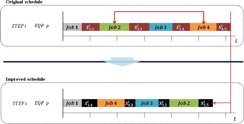
The following image powerfully illustrates this. By simply re-ordering the jobs, the setup times change, leading to a reduction in the total makespan.

Impact of Job Sequencing on Schedule with Sequence-Dependent Setup Times — This Gantt chart shows two schedules for the same four jobs. In the "Original schedule," the sequence is Job 1 -> 2 -> 3 -> 4. In the "Improved schedule," the sequence is changed to Job 1 -> 4 -> 3 -> 2. Notice how the setup times (the blocks between jobs) change with the sequence, resulting in a shorter overall makespan (completion time of the last job) for the improved schedule. This is the essence of sequence-dependent setups.

Formal Notation

In scheduling literature, these setup types are specified in the $β$ field of the standard $α ∣ β ∣ γ$ notation, which you learned in our first module.

STsi: denotes sequence-independent setup times.
STsd: denotes sequence-dependent setup times.

For example, a three-machine flow shop problem to minimize makespan with sequence-dependent setup times would be denoted as F3|STsd|Cmax. Recognizing this notation will be vital as you review literature for your thesis.

Test your understanding!

Imagine you need to schedule 3 jobs (J1, J2, J3) on a single machine. The processing times are $p_{1} = 10$ , $p_{2} = 15$ , and $p_{3} = 12$ . The setup from an idle state to the first job is 5 for any job.

Scenario A: The setup times are given by the following table. The time depends only on the job being set up ("To Job").

From Job	To J1	To J2	To J3
Any	4	6	3

Scenario B: The setup times are given by the following matrix, depending on both the "From Job" and "To Job".

From / To	J1	J2	J3
J1	-	12	5
J2	3	-	14
J3	8	4	-

Which scenario describes sequence-independent setups, and which describes sequence-dependent setups?
For Scenario A, what is the makespan for the sequence J2 -> J1 -> J3?
For Scenario B, what is the makespan for the sequence J2 -> J1 -> J3?
Now, for Scenario B, calculate the makespan for a different sequence: J1 -> J3 -> J2. How does it compare to the previous sequence's makespan? What does this demonstrate?

Show answer

Scenario A describes sequence-independent setup times because the setup time only depends on the "To Job". Scenario B describes sequence-dependent setup times because the setup time depends on both the "From Job" and the "To Job".
Scenario A (J2 -> J1 -> J3):
- Setup for J2 (from idle): 5
- Process J2: 15
- Setup for J1: 4 (from s_1=4)
- Process J1: 10
- Setup for J3: 3 (from s_3=3)
- Process J3: 12
- Total Makespan = 5 + 15 + 4 + 10 + 3 + 12 = 49
- Alternatively, using effective processing times: (5+15) + (4+10) + (3+12) = 20 + 14 + 15 = 49.
Scenario B (J2 -> J1 -> J3):
- Setup for J2 (from idle): 5
- Process J2: 15
- Setup from J2 to J1: 3 (from matrix s_21=3)
- Process J1: 10
- Setup from J1 to J3: 5 (from matrix s_13=5)
- Process J3: 12
- Total Makespan = 5 + 15 + 3 + 10 + 5 + 12 = 50
Scenario B (J1 -> J3 -> J2):
- Setup for J1 (from idle): 5
- Process J1: 10
- Setup from J1 to J3: 5 (from matrix s_13=5)
- Process J3: 12
- Setup from J3 to J2: 4 (from matrix s_32=4)
- Process J2: 15
- Total Makespan = 5 + 10 + 5 + 12 + 4 + 15 = 51
- The makespan for J1 -> J3 -> J2 is 51, which is different from the makespan of 50 for J2 -> J1 -> J3. This clearly demonstrates that for sequence-dependent setups, the choice of sequence directly affects the total time required.

Conclusion

In this lesson, we have established the crucial difference between two types of setup times, a concept that adds a significant layer of realism to scheduling models.

Key Takeaways:

Sequence-Independent Setup Time (STsi): Depends only on the job being prepared. Can often be absorbed into the processing time for simpler models.
Sequence-Dependent Setup Time (STsd): Depends on both the preceding and current jobs ( $s_{ij}$ ). It cannot be absorbed into processing time and makes finding an optimal sequence much harder, often introducing a TSP-like structure to the problem.
The choice between these two models has profound implications for problem complexity and the solution methods required.

Preview of the Next Lesson:

Understanding what these setups are is the first step. The next is to model them. In our next lesson, we will focus on the more challenging case: sequence-dependent setups. We will learn how to incorporate sequence-dependent setup times into MILP models, extending the formulations we've already built to handle this new, complex constraint.

Recommended resources