Common Scheduling Objectives

Hello! Welcome to our third lesson in the Foundations of Scheduling Theory.

In our last lesson, we defined release dates, due dates, and deadlines, establishing the time-based constraints that shape scheduling problems. We saw that due dates, in particular, serve as performance targets and are the foundation for metrics like lateness and tardiness.

Today, we will build directly on that by taking a comprehensive look at the most common scheduling objectives used in the γ field of our α|β|γ notation. The goal of this lesson is to help you distinguish between common scheduling objectives: makespan, total completion time, tardiness, and lateness. Understanding the trade-offs between these objectives is a critical first step in selecting the right approach for solving a real-world problem.

For an industrial engineer, choosing an objective is not just a mathematical exercise; it's a business decision that prioritizes a specific strategic goal. We can group these goals into three main categories, which will provide a structure for our lesson.

PRINCIPLES OF SEQUENCING AND SCHEDULING

To frame our discussion, please read this short excerpt from the textbook Principles of Sequencing and Scheduling by Baker and Trietsch. It introduces three prevalent decision-making goals in scheduling.

Read the second paragraph in the section '1.2 SCHEDULING THEORY', starting with 'Ideally, the objective function...' and ending with '...make these three goals operational.' This will introduce the concepts of throughput, turnaround, and timeliness.

As you just read, most scheduling objectives can be tied to one of three high-level goals:

Throughput: Maximizing the output of the system.
Turnaround: Minimizing the time jobs spend in the system.
Timeliness: Meeting committed due dates.

Let's now explore the specific objective functions associated with each of these goals.

1. Throughput: Makespan ( $C_{ma x}$ )

The objective most directly related to throughput is the makespan, denoted as $C_{ma x}$ .

Definition: Makespan is the time at which the last job completes processing. It is the time elapsed from the start of the first job to the completion of the last job in a schedule.

Mathematically, if $C_{j}$ is the completion time of job $j$ , then:
$C_{ma x} = max_{j} {C_{j}}$

Chapter 2

This chapter from a scheduling textbook provides a formal definition of makespan and explains its practical importance.

Please read the subsections 'Completion Times' and 'Makespan' near the beginning of the document. Then, read the paragraph under '2.3 Performance Measures' that starts with 'Most performance measures discussed in this book are regular. Actually, we have already seen one, the makespan Cmax.' Focus on how minimizing makespan relates to maximizing throughput and utilization.

As the text highlights, minimizing makespan is equivalent to maximizing the overall throughput of the facility. It answers the question: "How quickly can we finish this entire batch of work?" From a management perspective, this means the equipment and personnel will be free sooner to start the next batch of jobs, thereby maximizing the utilization of your resources. This is a system-focused objective.

Example: Calculating Makespan

Consider three jobs with the following processing times ( $p_{j}$ ):

Job 1: $p_{1} = 5$
Job 2: $p_{2} = 8$
Job 3: $p_{3} = 4$

If we process them in the sequence 1 -> 2 -> 3 on a single machine, starting at time 0:

Job 1 completes at $C_{1} = 5$ .
Job 2 completes at $C_{2} = 5 + 8 = 13$ .
Job 3 completes at $C_{3} = 13 + 4 = 17$ .

The completion times are {5, 13, 17}. The makespan is $C_{ma x} = max {5, 13, 17} = 17$ . Note that for a single machine with no idle time, the makespan is simply the sum of all processing times, regardless of the sequence. This changes in more complex environments like the flow shops and job shops we will study later.

2. Turnaround: Total Completion Time (or Flowtime)

While makespan looks at the system as a whole, objectives based on completion time or flowtime focus on the experience of individual jobs.

Definitions:

Completion Time ( $C_{j}$ ): The time at which job $j$ is finished.
Flowtime ( $F_{j}$ ): The total time job $j$ spends in the system, from its release until its completion. $F_{j} = C_{j} - r_{j}$ . When all jobs are available at time 0 ( $r_{j} = 0$ ), flowtime is identical to completion time.
Total Completion Time: The sum of the completion times of all jobs, $\sum_{j = 1}^{n} C_{j}$ . Minimizing this is equivalent to minimizing the average completion time.

Chapter 2

Let's return to the textbook chapter to explore the significance of this objective. It draws a crucial connection to a fundamental concept in industrial engineering.

Read section '2.4 Total completion time', stopping before '2.4.2 Complexity of the WSPT-rule'. Pay close attention to the relationship between total completion time, waiting times, and in-process inventory (Little's Law). The WSPT/SPT rules mentioned are optimization methods we will cover later; for now, focus on understanding the objective itself.

As you've read, minimizing total completion time has a powerful financial and operational implication: it minimizes the average work-in-process (WIP) inventory. According to Little's Law ( $L = λW$ ), the average number of jobs in the system ( $L$ ) is proportional to the average time a job spends in the system ( $W$ , or average flowtime). By reducing the total completion time, you reduce the average time each job is sitting in your facility, which in turn cuts down on inventory holding costs and improves system responsiveness. This is a job-focused or customer-focused objective.

3. Timeliness: Lateness and Tardiness

Timeliness objectives measure performance relative to a pre-defined target: the due date ( $d_{j}$ ).

Definitions:

Lateness ( $L_{j}$ ): The difference between a job's completion time and its due date. It can be positive (late), negative (early), or zero.
$L_{j} = C_{j} - d_{j}$
Tardiness ( $T_{j}$ ): The lateness of a job if it is late, and zero otherwise. It is always non-negative.
$T_{j} = max (0, L_{j}) = max (0, C_{j} - d_{j})$

The key distinction is that tardiness only penalizes lateness, while lateness considers both earliness and lateness. In most practical settings, tardiness is the more relevant measure because there is a cost for being late but often no reward for being early. (In Just-In-Time systems, however, earliness also has a cost related to inventory).

From these basic measures, we derive several common aggregate objectives:

Maximum Lateness ( $L_{ma x}$ ) or Maximum Tardiness ( $T_{ma x}$ ): $max_{j} L_{j}$ or $max_{j} T_{j}$ . This objective aims to minimize the worst-case performance for any single job, improving fairness and ensuring no customer is left waiting an exceptionally long time.
Total Tardiness ( $\sum T_{j}$ ): This objective seeks to minimize the overall sum of lateness across all tardy jobs.
Number of Tardy Jobs ( $\sum U_{j}$ ): Here, $U_{j} = 1$ if $T_{j} > 0$ and 0 otherwise. This objective simply tries to complete as many jobs as possible on time, regardless of how late the tardy jobs are.

Chapter 2

This last reading selection formally defines these timeliness-related objectives.

Read the sections '2.5 Lateness' (up to 2.5.2) and '2.6 Tardiness' (up to 2.6.1). This will solidify the definitions and distinctions between Lateness, Earliness, and Tardiness, and introduce the related objective functions.

Comparing the Objectives: An Example

The choice of objective function is critical because a schedule that is optimal for one objective may be very poor for another.

Let's examine a single schedule and evaluate it using multiple objectives. The image below shows a sequence for six jobs and calculates several performance metrics.

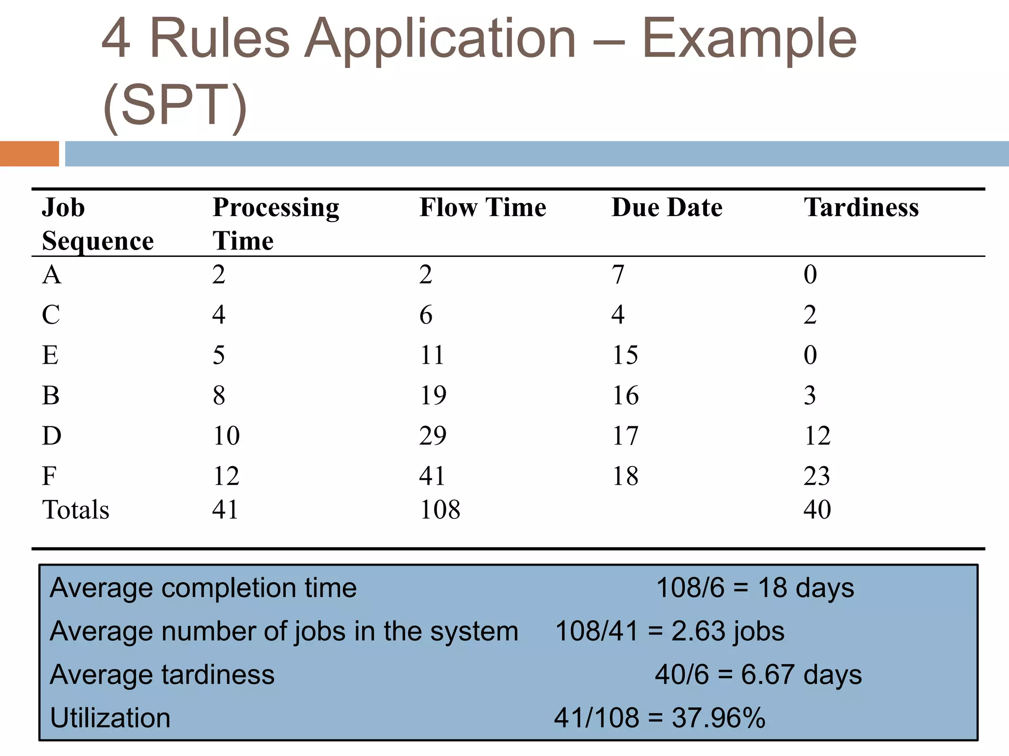
SPT Rule Application Example — This table illustrates the calculation of scheduling metrics for a sequence of jobs (A, C, E, B, D, F). For each job, it lists its processing time, completion time (Flow Time), due date, and resulting tardiness. Below the table, key metrics are calculated.

Let's analyze the results from the image for the sequence A -> C -> E -> B -> D -> F:

Makespan ( $C_{ma x}$ ): The last job, F, finishes at time 31. So, $C_{ma x} = 31$ .
Total Completion Time ( $\sum C_{j}$ ): The completion times (Flow Times) are 2, 5, 9, 15, 23, and 31.
$\sum C_{j} = 2 + 5 + 9 + 15 + 23 + 31 = 85$
The Average Completion Time is $85/6 \approx 14.17$ .
Maximum Tardiness ( $T_{ma x}$ ): The tardiness values for each job are 0, 0, 1, 7, 8, and 1. The maximum of these is 8 (for Job D). So, $T_{ma x} = 8$ .
Total Tardiness ( $\sum T_{j}$ ): The sum of the tardiness values is:
$\sum T_{j} = 0 + 0 + 1 + 7 + 8 + 1 = 17$
The Average Tardiness is $17/6 \approx 2.83$ .

This example demonstrates that for a single schedule, we can measure performance in fundamentally different ways, each corresponding to a different business priority.

Test your understanding!

Consider a single machine and the following four jobs.

Job (j)	Processing Time ( $p_{j}$ )	Due Date ( $d_{j}$ )
1	10	15
2	3	8
3	7	20
4	5	25

Let's compare two different sequences:

Sequence A: 1 -> 2 -> 3 -> 4
Sequence B: 2 -> 4 -> 3 -> 1

Calculate the four objective values ( $C_{ma x}$ , $\sum C_{j}$ , $T_{ma x}$ , $\sum T_{j}$ ) for each sequence. Which sequence is better for each objective?

Show answer

First, let's calculate the completion times and tardiness for each sequence.

Sequence A: 1 -> 2 -> 3 -> 4

Job (j)	$p_{j}$	$d_{j}$	$C_{j}$	$T_{j} = max (0, C_{j} - d_{j})$
1	10	15	10	0
2	3	8	13	5
3	7	20	20	0
4	5	25	25	0

$C_{ma x}$ : $max {10, 13, 20, 25} = 25$
$\sum C_{j}$ : $10 + 13 + 20 + 25 = 68$
$T_{ma x}$ : $max {0, 5, 0, 0} = 5$
$\sum T_{j}$ : $0 + 5 + 0 + 0 = 5$

Sequence B: 2 -> 4 -> 3 -> 1

Job (j)	$p_{j}$	$d_{j}$	$C_{j}$	$T_{j} = max (0, C_{j} - d_{j})$
2	3	8	3	0
4	5	25	8	0
3	7	20	15	0
1	10	15	25	10

$C_{ma x}$ : $max {3, 8, 15, 25} = 25$
$\sum C_{j}$ : $3 + 8 + 15 + 25 = 51$
$T_{ma x}$ : $max {0, 0, 0, 10} = 10$
$\sum T_{j}$ : $0 + 0 + 0 + 10 = 10$

Comparison:

Makespan: Both sequences have the same makespan (25), which is expected for a single machine.
Total Completion Time: Sequence B (51) is better than Sequence A (68). This means Sequence B results in lower average WIP inventory.
Maximum Tardiness: Sequence A (5) is better than Sequence B (10). Sequence A is "fairer" to all jobs.
Total Tardiness: Sequence A (5) is better than Sequence B (10). Sequence A incurs a lower total lateness penalty.

This clearly shows the trade-off: Sequence B is better for internal efficiency (inventory), while Sequence A is better for customer satisfaction (timeliness).

Conclusion

In this lesson, we have defined, calculated, and contrasted the primary scheduling objectives. Here are the key takeaways:

Makespan ( $C_{ma x}$ ): A system-level objective focused on throughput and resource utilization.
Total Completion Time ( $\sum C_{j}$ ): A job-level objective focused on turnaround and minimizing work-in-process inventory.
Lateness ( $L_{j}$ ): Measures deviation from a due date, can be positive or negative.
Tardiness ( $T_{j}$ ): Measures only how late a job is ( $T_{j} \geq 0$ ). Objectives based on tardiness ( $T_{ma x}$ , $\sum T_{j}$ ) are focused on timeliness and customer satisfaction.

You now have a solid understanding of what we are trying to optimize in a scheduling problem. This knowledge is the final pillar of the α|β|γ framework.

Preview of the next lesson: In our next module, "Single Machine Scheduling," we will move from defining objectives to actively optimizing for them. We will start by learning how to find the optimal sequence that minimizes total completion time on a single machine using the Shortest Processing Time (SPT) rule. This will be your first look at a provably optimal scheduling algorithm.

Recommended resources

1. Throughput: Makespan (Cmax​)

Example: Calculating Makespan

2. Turnaround: Total Completion Time (or Flowtime)

3. Timeliness: Lateness and Tardiness

Comparing the Objectives: An Example

Conclusion

1. Throughput: Makespan ( $C_{ma x}$ )