Hello! In our first lesson, we established the α|β|γ notation as the universal language for describing scheduling problems. This framework allows us to precisely define the machine environment, job characteristics, and optimization goals.
Today, we'll build on that foundation by taking a closer look at some of the most critical time-based constraints and targets that appear in the β and γ fields. Specifically, this lesson will describe the role of release dates, due dates, and deadlines in scheduling. Understanding these concepts is fundamental, as they introduce the real-world complexities of job availability and delivery commitments into our mathematical models.
Recap: Time Constraints in α|β|γ Notation
Recall from our previous lesson:
- The
βfield describes job characteristics. The termr_jsignifies that jobs have release dates. - The
γfield defines the objective function. Objectives likeL_max(maximum lateness) or∑T_j(total tardiness) are directly related to due dates.
Let's now formally define these terms and explore their impact on scheduling problems.
1. Release Dates: When Can a Job Start?
A release date, denoted as , is the earliest time at which job becomes available for processing. Before its release date, a job simply cannot be scheduled, even if a machine is free.
In many real-world scenarios, jobs are not all available at the beginning of the planning horizon. For example, in a factory setting, raw materials for a specific job might not arrive until a certain time. In a computing environment, a task might depend on the output of a process that finishes at a specific time.
Scheduling Algorithms 1 Introduction - People
For a formal introduction to this concept, let's turn to the paper 'Scheduling Algorithms' by Karger et al.
Please read the first paragraph under the heading 'A number of side constraints...'. This section formally introduces release date constraints within the scheduling framework.
The Role of Release Dates
The primary role of release dates is to constrain the set of schedulable jobs at any point in time.
- Default Assumption: If
r_jis not mentioned in a problem'sβfield, it's assumed that all jobs are available at time 0 ( for all ). - Introducing Idle Time: When non-trivial release dates exist, it may be optimal for a machine to remain idle, waiting for a high-priority job to be released, rather than immediately starting a currently available but lower-priority job.
- Increasing Complexity: The introduction of release dates can dramatically increase the computational complexity of a scheduling problem. Many problems that are easy to solve when all jobs are available at time 0 become NP-hard when release dates are added. We will see a concrete example of this shortly.
2. Due Dates and Deadlines: When Should a Job Finish?
While release dates constrain the start of a job, due dates and deadlines relate to its completion. It's crucial to distinguish between these two terms.
- A due date () is a target completion time for job . Finishing after the due date is undesirable and usually incurs a penalty, but it is not forbidden.
- A deadline () is a hard constraint. Job must be completed by time . Any schedule that violates a deadline is considered infeasible. In the
α|β|γnotation, deadlines are often modeled as a special type of constraint in theβfield, while due dates are typically used to define the objective function in theγfield.
In your industrial engineering context, due dates represent commitments to customers, while deadlines might represent physical constraints, such as a chemical that will spoil if not processed by a certain time.
The Role of Due Dates: Defining Performance
The primary role of due dates is to provide a reference point for measuring the timeliness of a schedule. From due dates, we derive several key performance metrics.
The following lecture notes provide clear, concise definitions for the key parameters derived from due dates.
First, review the 'Parameters of scheduling problems' table, focusing on the definitions for Lateness and Tardiness. Then, read the section 'The engineering meaning of the objective functions' to understand how these metrics are used.
Let be the completion time of job . The most important metrics related to its due date are:
- Lateness (): Defined as .
- If , the job is tardy or late.
- If , the job is early.
- If , the job is on time.
- Tardiness (): Defined as .
- Tardiness is always non-negative. It measures how late a tardy job is and ignores any earliness. This is often more practical, as there's usually a cost for being late but no reward for being early.
- Earliness (): Defined as .
- This measures how early a job is completed. In just-in-time (JIT) systems, both earliness (which increases inventory costs) and tardiness are penalized.
These job-level metrics are then aggregated into objective functions for the γ field, such as:
L_max: Minimize the maximum lateness (). This focuses on the worst-case performance, aiming to ensure no single job is excessively late.∑T_j: Minimize the sum of tardiness. This aims to reduce the total amount of lateness across all jobs.∑U_j: Minimize the number of tardy jobs, where is 1 if job is tardy () and 0 otherwise.
A Concrete Example
Let's look at how these values are calculated. The table below shows a schedule for six jobs, ordered by the Shortest Processing Time (SPT) rule. "Flow time" is another term for completion time ().
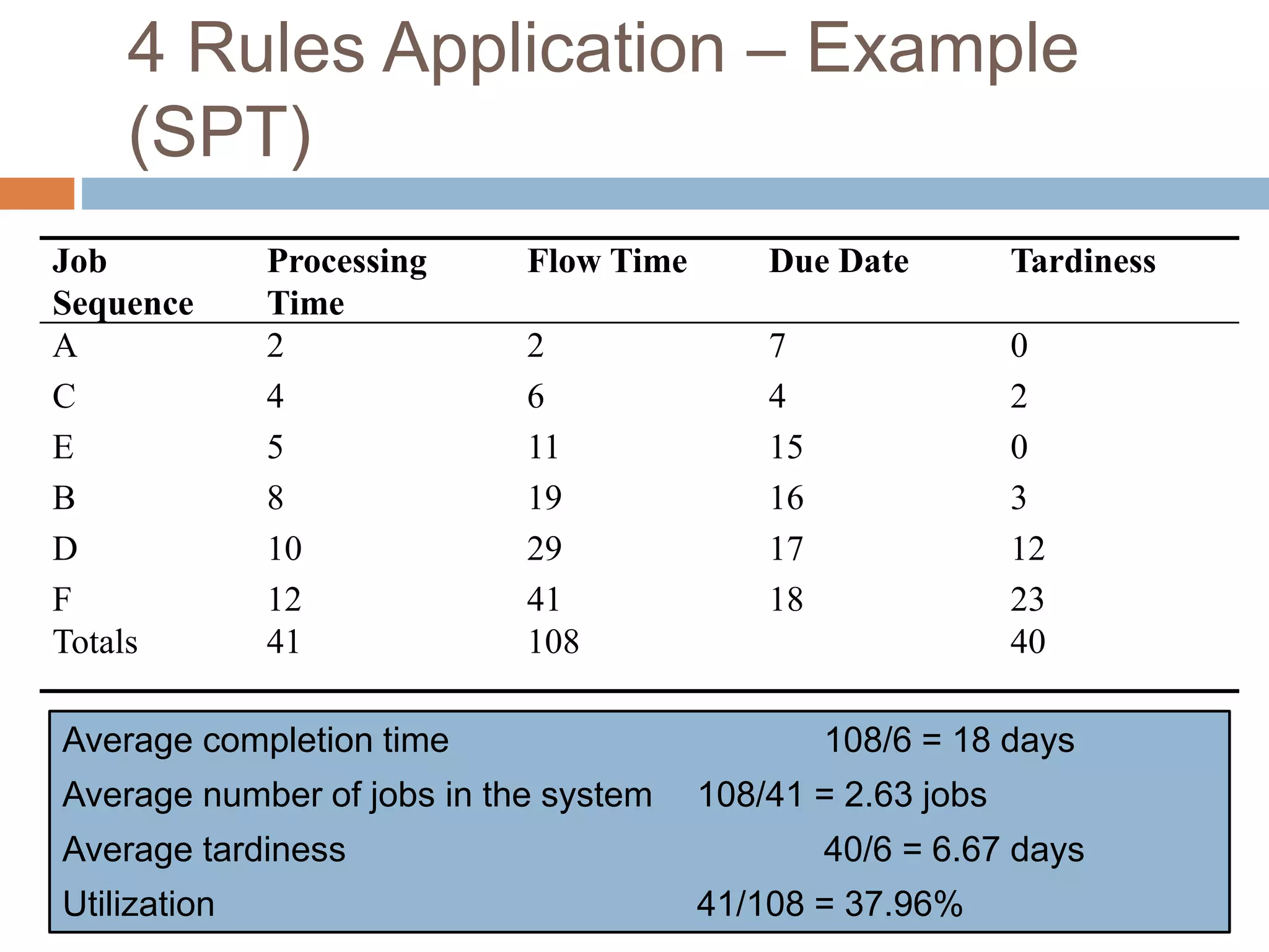
Let's trace the calculation for Job B:
- Sequence: Jobs are processed in the order A, C, E, B, D, F.
- Completion Time (): Job A takes 2 hours, C takes 3, and E takes 4. Job B starts after E finishes at time 9 and takes 6 hours. So, .
- Due Date (): The table states the due date for Job B is 8.
- Lateness (): . Job B is 7 hours late.
- Tardiness (): .
As you can see, the due date acts as the benchmark against which the schedule's performance is measured.
Test your understanding!
Consider a single machine and the following three jobs:
| Job (j) | Processing Time () | Release Date () | Due Date () |
|---|---|---|---|
| 1 | 5 | 0 | 8 |
| 2 | 4 | 2 | 10 |
| 3 | 6 | 0 | 15 |
Suppose the jobs are scheduled in the sequence 3 -> 1 -> 2.
- Is this sequence valid, considering the release dates? Why or why not?
- If valid, calculate the completion time (), lateness (), and tardiness () for each job.
- What are the values for
L_maxand∑T_jfor this sequence?
Show answer
-
Validity: Yes, the sequence is valid. Job 3 can start at time 0. Job 1 can start after Job 3 finishes. Job 2 is released at time 2, but it is scheduled to start much later, so its release date is respected.
-
Calculations:
- Job 3: Starts at 0, finishes at .
- (9 units early)
- Job 1: Starts at 6 (when Job 3 finishes), finishes at .
- (3 units tardy)
- Job 2: Starts at 11 (when Job 1 finishes), finishes at .
- (5 units tardy)
- Job 3: Starts at 0, finishes at .
-
Objective Values:
L_max: The lateness values are . The maximum is 5. So,L_max= 5.∑T_j: The tardiness values are . The sum is . So,∑T_j= 8.
Conclusion
In this lesson, we have formally defined and examined the roles of three fundamental time-based concepts in scheduling:
- Release Dates (): Act as availability constraints, dictating the earliest start time for a job. They are part of the problem definition (
βfield) and can significantly increase scheduling complexity. - Due Dates (): Serve as performance targets. They are used to calculate lateness and tardiness, which form the basis for many common objective functions (
γfield). - Deadlines (): Are hard constraints that define the latest possible completion time for a job. Violating a deadline results in an infeasible schedule.
You now understand how these elements move us from simple sequencing to more realistic and challenging time-constrained optimization problems, which are at the heart of scheduling research and practice.
In the next lesson, we will continue our exploration of core concepts by comparing and contrasting the most common scheduling objectives we introduced today, such as makespan (C_max), total completion time (∑C_j), and various due-date-related metrics. This will help you understand the trade-offs involved in choosing an objective for a given industrial problem.