Introduction to Scheduling Problems: α|β|γ Notation

What is a Scheduling Problem?

At its core, scheduling is about making decisions. Specifically, it involves assigning limited resources to a set of tasks or activities over time, with the goal of achieving a specific objective.

As the presentation highlights, any scheduling problem can be broken down into three components:

1. Resources: The machines, workers, or processors that perform the tasks.
2. Tasks: The jobs or operations that need to be completed.
3. Objective: The goal we want to achieve, such as minimizing cost, time, or maximizing productivity.

To communicate these three components concisely, researchers use a standardized notation.

The Standard Three-Field Notation: α|β|γ

In the 1970s, a team of researchers including Ronald Graham proposed a simple and powerful notation to classify the vast landscape of scheduling problems. This is now universally known as the α|β|γ notation.

• α (alpha) describes the machine environment (the resources).
• β (beta) describes the job characteristics and constraints (the tasks).
• γ (gamma) describes the objective function to be minimized or maximized.

Let's break down each field. For a comprehensive reference, we will use the following resource.

The α Field: Machine Environment

The α field tells us about the machines we are scheduling on.

Here is a summary of the most common entries for the α field:

• 1: A single machine. This is the simplest environment.
• P: Identical parallel machines. Any job can be processed on any machine, and the processing time is the same on all of them. P2 would mean there are exactly two such machines.
• Q: Uniform parallel machines. Machines have different speeds. A machine i with speed s_i would process job j in p_j / s_i time.
• R: Unrelated parallel machines. The processing time of job j depends on the specific machine i it is assigned to, denoted p_{ij}. There's no simple speed relationship.
• F: Flow Shop. Jobs must pass through a series of machines in the same order. A classic assembly line is a flow shop. F2 means a two-machine flow shop.
• J: Job Shop. Each job has its own specific route through the machines. Unlike a flow shop, different jobs can have different routes.
• O: Open Shop. Each job has a set of operations, each on a different machine, but these operations can be performed in any order.

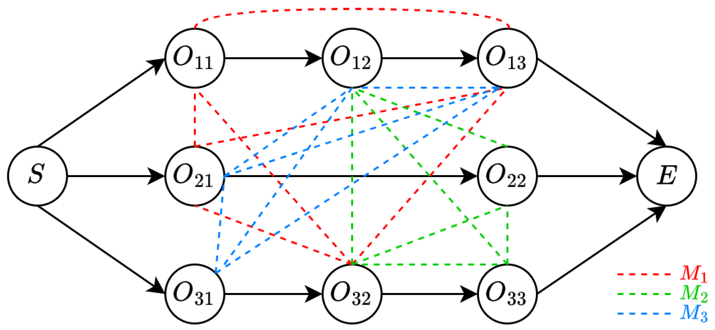
Your thesis focuses on the Flexible Job Shop Problem (FJSP). In the standard notation, this is often indicated by the term rcrc (recirculation) in the β field, which relaxes the job shop constraint that each operation has a dedicated machine. The flexibility means an operation can be processed by one of several alternative machines.

The β Field: Job Characteristics

The β field specifies the constraints and characteristics of the jobs. If this field is empty, it implies a set of standard default assumptions (e.g., all jobs are available at time zero, no preemption, etc.).

Here are some key entries for the β field:

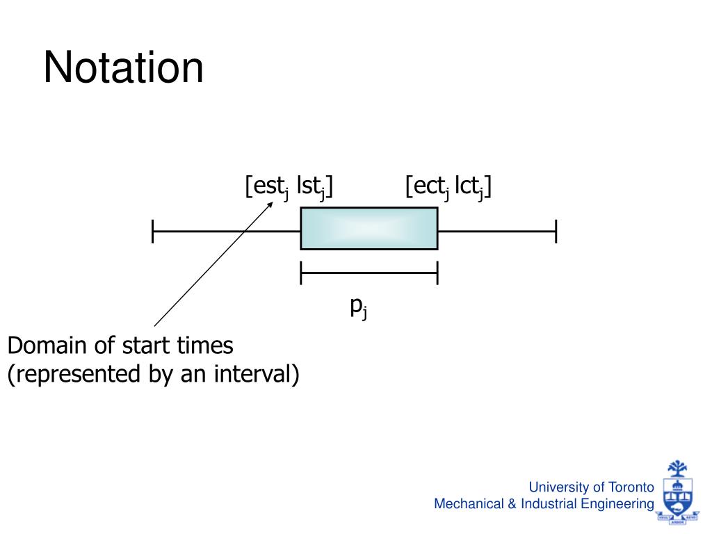
• p_j=1 or p_j=p: All jobs have unit processing time or equal processing time, respectively.
• r_j: Jobs have release dates. A job j cannot start before its release date r_j.
• d_j: Jobs have due dates. This is often implied and used by the objective function. We will discuss this more in the next lesson.
• pmtn: Preemption is allowed. A job can be interrupted and resumed later, possibly on a different machine, without penalty. The default is non-preemption.
• prec: Jobs are subject to precedence constraints. This is typically represented as a directed acyclic graph where an arc from job i to j means i must be completed before j can start.
• no-wait: A job, once started, must be processed continuously through all its machine stages without any waiting time between operations.
• t_jk: Transportation delays exist between machines, a key factor in realistic manufacturing environments and relevant to your future work on complex constraints.

The γ Field: Objective Function

The γ field defines the performance measure we want to optimize, which is usually minimization.

Here are the most common objectives:

• C_max: Minimize the Makespan. This is the time when the last job finishes, i.e., max(C_j) over all jobs j. Minimizing makespan is equivalent to maximizing the overall throughput of the system.
• ∑C_j: Minimize the Total Completion Time (or sum of completion times). This objective aims to get all jobs finished quickly on average, which reduces work-in-process inventory.
• L_max: Minimize the Maximum Lateness. Lateness of a job j is L_j = C_j - d_j. This can be positive (tardy) or negative (early). Minimizing the maximum lateness is important for meeting service level agreements where the worst-case performance matters most.
• ∑T_j: Minimize the Total Tardiness. Tardiness is T_j = max(0, C_j - d_j). Unlike lateness, it only penalizes jobs that are late. This is a common objective when there is a cost associated with being late but no benefit for being early.
• ∑w_j C_j: Minimize the Total Weighted Completion Time. Here, each job has a weight w_j representing its importance. This is useful for prioritizing critical jobs.

Putting It All Together: Examples

Let's see how these fields combine to precisely define a scheduling problem.

• 1 | r_j | L_max: This describes a problem on a single machine (1), where jobs have release dates (r_j), and the goal is to minimize the maximum lateness (L_max).
• P | | C_max: This is a problem on multiple identical parallel machines (P), with no special constraints (the β field is empty), and the objective is to minimize the makespan (C_max).
• F2 | | C_max: This is the classic two-machine flow shop problem where the goal is to minimize the makespan. We will study the efficient solution for this, Johnson's algorithm, in Module 3.
• Jm | | C_max: This describes the general m-machine job shop problem with the objective of minimizing the makespan. This is a famously difficult problem and a precursor to your thesis topic.

Conclusion

In this lesson, we have introduced the fundamental α|β|γ notation, which is the standard language of scheduling theory. You learned how to describe the three core components of any scheduling problem:

• The machine environment (α), from single machines to complex job shops.
• The job characteristics (β), including timing constraints and preemption rules.
• The objective function (γ), such as minimizing makespan or tardiness.

Mastering this notation is the first and most critical step in your journey. It will allow you to precisely define problems and navigate the vast body of research literature relevant to your thesis.

In the next lesson, we will delve deeper into the concepts mentioned in the β and γ fields. We will formally define release dates, due dates, and deadlines, and we'll take a closer look at the common scheduling objectives we'll be trying to optimize throughout this course.