Preemptive vs. Non-Preemptive Scheduling

1. The Core Distinction: To Interrupt or Not to Interrupt

At its heart, the difference is simple:

• Non-Preemptive Scheduling: Once a machine starts processing a job, it must continue until the job is fully completed. The job cannot be interrupted. This is the default assumption in many manufacturing and scheduling environments.
• Preemptive Scheduling: A job currently being processed can be interrupted (preempted) and set aside. The machine can then start working on a different job. The preempted job can be resumed later, either from where it left off or after some setup.

This diagram provides a clear visual representation of the concept.

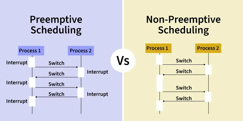
As you can see, preemption allows for dynamic switching between tasks, while non-preemption enforces a "run-to-completion" policy.

To solidify these definitions and see how they are applied, let's watch a short video. It uses computer science terminology (e.g., 'CPU', 'process'), but the underlying logic is identical to scheduling jobs on machines.

2. Formalizing the Concept and Its Implications

In the α|β|γ notation, the presence of preemption is indicated by prmp in the β field. If prmp is not listed, the scheduling environment is assumed to be non-preemptive.

The choice between these two modes involves a critical trade-off:

• Flexibility vs. Overhead: Preemption offers the flexibility to respond to urgent or high-priority jobs as soon as they arrive. However, this flexibility comes at a cost. In manufacturing, this "overhead" isn't just computational; it can involve physical setup times to switch between jobs (e.g., cleaning, retooling, or recalibrating a machine), which can be very expensive and time-consuming.
• Optimality and Complexity: The most profound implication of preemption lies in its effect on problem complexity. A scheduling problem that is computationally "hard" (NP-hard) in a non-preemptive environment can sometimes become "easy" (polynomially solvable) if preemption is allowed.

Let's look at a concrete example from an academic resource.

This is a powerful result. By simply allowing interruptions, a problem that is intractable for large instances becomes efficiently solvable. This happens because preemption gives the scheduler the freedom to immediately address a job that is about to become late, without being 'stuck' finishing a less urgent job that started earlier.

3. Preemptive Scheduling Rules

When preemption is allowed, we often use different scheduling rules that take advantage of this capability. These rules typically check at every decision point (e.g., when a new job arrives or a job completes) whether the currently running job is still the best one to be processing.

Some common preemptive rules include:

• Shortest Remaining Processing Time (SRPT): This is the preemptive version of the Shortest Processing Time (SPT) rule. When a new job arrives, the scheduler compares its processing time to the remaining processing time of the job currently on the machine. If the new job is shorter, it preempts the current job. The video you watched referred to this as "Shortest Remaining Job First".
• Preemptive Earliest Due Date (EDD): As seen in the reading, this rule is optimal for the 1 | rj, prmp | Lmax problem. At any point in time, the machine works on the available job with the earliest due date.
• Longest Remaining Processing Time (LRPT): This is the preemptive version of the Longest Processing Time (LPT) heuristic. It is notable because it provides an optimal solution for the Pm | prmp | Cmax problem (minimizing makespan on parallel machines with preemption), further highlighting how preemption can lead to powerful, optimal algorithms.

Conclusion

You should now have a clear understanding of the fundamental differences between preemptive and non-preemptive scheduling.

Key Takeaways:

• Non-Preemptive: A job, once started, runs to completion without interruption. This is simpler and avoids the overhead of switching tasks.
• Preemptive: A running job can be interrupted to process another, more urgent job. This provides flexibility and can significantly improve performance for certain objectives (like minimizing lateness).
• Impact: The choice to allow preemption is a major structural decision. It can change a computationally hard problem into an easy one, but it comes with potential real-world costs (e.g., setup times).
• Relevance to Your Thesis: In the context of Flexible Job Shop Problems (FJSP), most standard models assume non-preemptive operations within a single machine. Preemption, if allowed, is a specific and important characteristic that must be explicitly modeled, often making the problem even more complex to represent and solve.

Preview of the next lesson: In this lesson, we encountered terms like "NP-complete" and "easy" problems. To properly understand what these mean and why they are so crucial for scheduling research, our next lesson will formally introduce the computational complexity classes (P, NP, NP-hard) relevant to scheduling. This will provide a rigorous foundation for classifying the difficulty of the problems you will face in your research.