Space Complexity: Understanding Memory Usage

1. What is Space Complexity?

While time complexity measures how many operations an algorithm performs, space complexity measures the amount of memory an algorithm needs to run as a function of its input size.

In an interview context, it's crucial to distinguish between two components of an algorithm's memory usage.

1. Input Space: The memory used to store the input data. For example, if your function receives a list of $n$ integers, the input space is proportional to $n$.
2. Auxiliary Space: This is the extra or temporary memory that the algorithm allocates while it runs. This includes new data structures it creates or space used by function calls (which we'll explore more with recursion).

In most technical interviews, when asked for "space complexity," the interviewer is interested in the auxiliary space complexity. They want to know how much additional memory your algorithm uses, beyond the space taken by the inputs.

As the article highlights, for a Data Engineer, optimizing for space can directly translate to cost savings in the cloud and enable the processing of massive datasets on hardware with finite memory.

2. The Components of Space Complexity

When calculating auxiliary space, we follow a similar logic to time complexity: we count what matters and ignore what doesn't. The video below provides a very clear, structured breakdown.

To summarize, when analyzing the auxiliary space of an iterative algorithm, we primarily focus on:

• Data Structures: Any new arrays, lists, sets, dictionaries, etc., that the algorithm creates.
• Variables: We generally ignore simple variables (integers, pointers) as they take up constant, $O(1)$, space.

Let's see a practical comparison of two approaches to the same problem, one that uses extra space and one that doesn't.

This concept of in-place algorithms (those with $O(1)$ auxiliary space) is extremely important. They are highly memory-efficient, which is a desirable quality for production code.

3. Common Space Complexity Classes

Just like with time, we use Big O notation to classify how an algorithm's memory usage scales. The growth rates are the same, but now they refer to memory instead of operations.

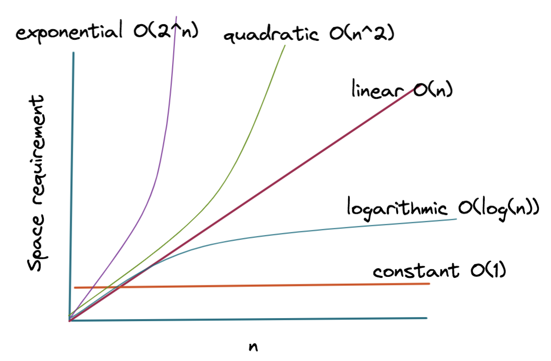
Let's look at the most common space complexity classes you'll encounter.

Here's a summary of the key classes from the article:

• $O(1)$ — Constant Space: The algorithm uses a fixed amount of memory regardless of the input size. This is the ideal for memory efficiency. Swapping two variables or iterating through an array with a few index variables are $O(1)$ space operations.

  # O(1) auxiliary space
  def get_max_element(numbers):
      max_val = numbers[0]
      # 'max_val' and 'num' are O(1) space
      for num in numbers:
          if num > max_val:
              max_val = num
      return max_val
  

• $O(n)$ — Linear Space: The extra memory used grows in direct proportion to the input size $n$. This often happens when you create a copy of the input or use a helper data structure that stores one element for each input element.

  # O(n) auxiliary space
  def reverse_list(numbers):
      # 'reversed_arr' grows with the size of 'numbers'
      reversed_arr = [] 
      for i in range(len(numbers) - 1, -1, -1):
          reversed_arr.append(numbers[i])
      return reversed_arr
  

• $O(\log n)$ — Logarithmic Space: Memory usage grows logarithmically with the input size. This is less common in iterative algorithms but is a key feature of the space complexity for certain recursive algorithms (like recursive binary search), where the number of nested function calls on the stack is $\log n$. We will revisit this in the recursion module.

• $O(n^2)$ — Quadratic Space: Memory usage is proportional to the square of the input size. A common example is creating an adjacency matrix to represent a graph with $n$ vertices, which requires an $n\times n$ grid.

4. The Time vs. Space Trade-off

Often, you can make an algorithm faster by using more memory, or make it more memory-efficient by accepting a slower runtime. This is known as the time-space trade-off, and it's a fundamental concept in algorithm design.

A classic interview example is finding a duplicate number in a list.

• Approach 1 (More Space, Less Time): Iterate through the list and store each number in a hash set. If you encounter a number that's already in the set, you've found a duplicate.

  • Time Complexity: $O(n)$, because you visit each element once.
  • Auxiliary Space Complexity: $O(n)$, because in the worst case, you store all $n$ elements in the hash set.

• Approach 2 (Less Space, More Time): For each element, iterate through the rest of the list to see if a duplicate exists.

  • Time Complexity: $O(n^2)$, due to the nested loop.
  • Auxiliary Space Complexity: $O(1)$, as you only use a few variables to keep track of indices.

Which approach is better? It depends on the constraints. If the input list is small, the $O(n^2)$ time might be acceptable. If the list is massive and you have plenty of RAM, the $O(n)$ time / $O(n)$ space solution is far superior. Recognizing and discussing these trade-offs is a sign of a mature problem-solver.

5. Practice: Your Turn to Analyze

Now, let's analyze the auxiliary space complexity of the following Python functions.

Problem 1:
A function that calculates the sum of a list of numbers.

def calculate_sum(numbers):
    total = 0 # One variable
    for num in numbers:
        total += num
    return total

Problem 2:
A function that finds all unique elements from a list.

def find_unique_elements(numbers):
    unique_set = set() # A new data structure
    for num in numbers:
        unique_set.add(num)
    
    # Convert set back to a list before returning
    return list(unique_set)

Problem 3:
A function that generates a list of all pairs from an input list.

def generate_all_pairs(items):
    n = len(items)
    pairs = [] # A new list to store pairs
    for i in range(n):
        for j in range(n):
            pairs.append((items[i], items[j]))
    return pairs

Conclusion

Fantastic work today. You have now learned about the second critical dimension of algorithm efficiency: space complexity.

Here are the main takeaways:

• Space Complexity measures an algorithm's memory usage as a function of its input size.
• Auxiliary Space is the extra memory used by an algorithm, and it's typically the focus of interview questions.
• We use Big O notation to classify space complexity, with common classes being $O(1)$ (constant), $O(n)$ (linear), and $O(\log n)$ (logarithmic).
• An in-place algorithm has an auxiliary space complexity of $O(1)$.
• There is often a time-space trade-off, where you can improve runtime at the cost of using more memory, or vice versa.

So far, we've discussed how to analyze the time and space complexity of algorithms in a general sense. But how efficient are the fundamental tools you use every day in Python? In our next lesson, we will analyze the time and space efficiency of Python's built-in list and dictionary operations, a crucial piece of knowledge for writing high-performance code.