Analyzing Loop Time Complexity

1. A Systematic Approach to Analyzing Loops

When you see a piece of code with loops, the goal is to count the total number of "basic operations" it performs in the worst case. A simple and effective strategy is:

1. Count the Iterations: Determine how many times the loop will run as a function of the input size, $n$.
2. Analyze the Loop Body: Determine the time complexity of the code inside the loop for a single iteration. This is often $O(1)$ if it involves simple arithmetic, assignments, or comparisons.
3. Multiply: The total time complexity is the (Number of Iterations) × (Complexity of the Loop Body).

Let's start by looking at some common loop patterns you'll encounter.

2. Single Loop Patterns

Linear Time: $O(n)$

This is the most common pattern. A loop's complexity is linear if its iteration count is directly proportional to the input size, $n$. This typically happens when the loop variable is incremented or decremented by a constant value in each step.

Consider this Python code:

# Assume 'data' is a list of size n
def process_data(data):
    # This loop runs n times
    for item in data:
        # Assume this is an O(1) operation
        print(item) 

Here, the loop runs len(data) times, which is $n$. The operation inside, print(item), takes constant time for each item.
Therefore, the total complexity is $n\times O(1)=O(n)$.

To see a practical demonstration of how linear time scales, let's watch a short video segment.

Logarithmic Time: $O(\log n)$

We touched on $O(\log n)$ last time with binary search. This highly efficient complexity often appears in loops where the control variable is multiplied or divided by a constant factor in each iteration. This pattern effectively shrinks the problem size exponentially.

Consider this loop:

def logarithmic_loop(n):
    i = 1
    while i < n:
        # O(1) operation
        print(i)
        i *= 2 # i is doubled in each iteration

How many times does this loop run?

• Iteration 1: i = 1
• Iteration 2: i = 2
• Iteration 3: i = 4
• Iteration 4: i = 8
• ...
• Iteration k: i = 2^(k-1)

The loop stops when $i\ge n$. Let's say it runs $k$ times. At the end, $i$ will be roughly equal to $n$. So, we have the equation $2^k\approx n$. To solve for $k$ (the number of iterations), we take the logarithm of both sides: $k\approx {\log }_{2}n$.

Since Big O notation ignores the base of the logarithm (it's just a constant factor), the complexity is $O(\log n)$.

For a detailed walkthrough of this analysis, the following video is excellent.

3. Nested Loop Patterns

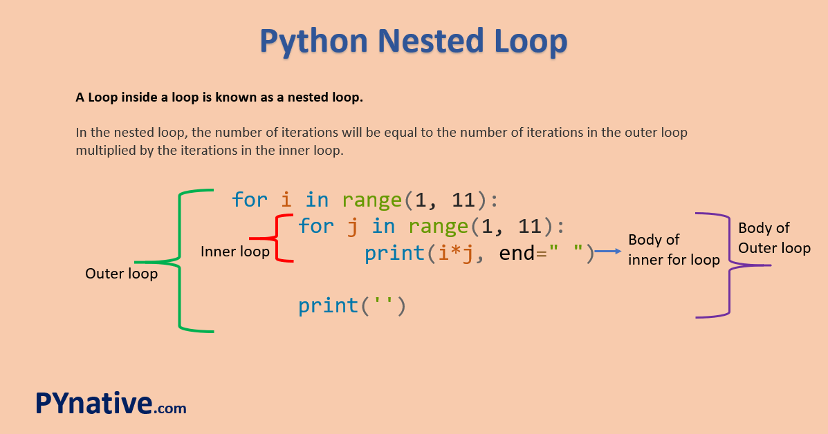
Nested loops are another very common structure, where one loop is placed inside another.

Quadratic Time: $O(n^2)$

This complexity often arises from a simple nested loop where both loops iterate roughly $n$ times.

def find_pairs(data):
    n = len(data)
    # Outer loop runs n times
    for i in range(n):
        # Inner loop also runs n times
        for j in range(n):
            # O(1) operation
            print(data[i], data[j])

Here, the outer loop runs $n$ times. For each of those $n$ iterations, the inner loop also runs $n$ times.

• Total Operations = (Outer Loop Iterations) × (Inner Loop Iterations) × (Loop Body Complexity)
• Total Operations = $n\times n\times O(1)=O(n^2)$

The following video again provides a great visualization of how quickly $O(n^2)$ runtimes grow compared to linear ones.

Dependent Nested Loops: Still $O(n^2)$!

A slightly trickier case is when the inner loop's iterations depend on the outer loop's variable.

def find_unique_pairs(data):
    n = len(data)
    # Outer loop runs n times
    for i in range(n):
        # Inner loop's iterations depend on 'i'
        for j in range(i + 1, n):
            # O(1) operation
            print(data[i], data[j])

Let's count the inner loop's iterations:

• When i = 0, inner loop runs $n-1$ times.
• When i = 1, inner loop runs $n-2$ times.
• ...
• When i = n-2, inner loop runs 1 time.
• When i = n-1, inner loop runs 0 times.

The total number of operations is the sum of an arithmetic series: $(n-1)+(n-2)+...+1+0$. This sum is equal to $\frac{n(n-1)}{2}=\frac{1}{2}{n}^2-\frac{1}{2}n$.

Following the rules of Big O, we drop the constants ($\frac{1}{2}$) and the lower-order term ($-\frac{1}{2}n$), which leaves us with $O(n^2)$.

The next video gives a fantastic, methodical explanation of how to analyze this exact pattern.

4. Combining Loops

What if loops aren't nested, but appear one after another?

Consecutive Loops: $O(m+n)$

When you have two separate, non-nested loops, you simply add their complexities.

def process_two_lists(list_m, list_n):
    # This loop runs m times, where m = len(list_m)
    for item in list_m:
        print(item) # O(1)

    # This loop runs n times, where n = len(list_n)
    for item in list_n:
        print(item) # O(1)

The total complexity is $O(m)+O(n)=O(m+n)$. If $m$ and $n$ are related (e.g., $m=n$), this simplifies to $O(n)+O(n)=O(2n)$, which we know is just $O(n)$.

To reinforce this, please read the following brief section.

5. Practice: Your Turn to Analyze

Now, let's put this into practice. Analyze the time complexity of the following Python functions. Frame your answer in terms of $n$, where $n$ is the size of the input list.

Problem 1:

def mystery_function_1(numbers):
    n = len(numbers)
    for i in range(n // 2):
        print(numbers[i])

Problem 2:

def mystery_function_2(n):
    count = 0
    i = n
    while i > 1:
        i = i // 3  # Integer division
        count += 1
    return count

Problem 3:

def mystery_function_3(numbers):
    n = len(numbers)
    for i in range(n):
        for j in range(n):
            for k in range(100): # A constant number of iterations
                if numbers[i] == numbers[j]:
                    return True
    return False

Conclusion

Great work! Today you've learned a structured approach to analyzing the time complexity of iterative code, a skill that is tested in almost every technical interview.

Here are the key patterns to remember:

• Single loop with constant step: $O(n)$
• Single loop with multiplicative/divisive step: $O(\log n)$
• Two simple nested loops: $O(n^2)$
• Two dependent nested loops (triangular iteration): $O(n^2)$
• Consecutive (sequential) loops: Add the complexities, e.g., $O(m+n)$, and keep the dominant term.

So far, we've focused entirely on time complexity. However, an algorithm's efficiency is also measured by how much memory it uses. In our next lesson, we will introduce space complexity, exploring how to analyze an algorithm's memory footprint and why it's a critical consideration, especially in data engineering where datasets can be massive.