Parametric Survival Models: Estimation and Interpretation

Introduction

In our previous lesson, we established the fundamental process for parametric survival analysis: constructing the likelihood function from data that includes censored observations. We saw that the likelihood is a product of probability densities $f (t)$ for events and survival probabilities $S (t)$ for right-censored observations.

This lesson takes the critical next step. We will now use the principle of maximum likelihood to fit parametric survival models to data. Your background as a statistician means you are already well-versed in Maximum Likelihood Estimation (MLE); our focus will be on its specific application and interpretation in the context of survival analysis. We will learn how to derive the estimators for model parameters, understand what those parameters tell us about the underlying failure process, and use statistical tests to compare different models.

We'll begin with the single-parameter exponential model to solidify the mechanics and then advance to the more flexible two-parameter Weibull model, which is a cornerstone of actuarial modeling.

The Principle of Maximum Likelihood Estimation in Survival Analysis

As you know, the core idea of MLE is to find the parameter values, $θ$ , that maximize the likelihood of observing the data we have collected. In survival analysis, this means maximizing the log-likelihood function we derived previously:

l (θ) = i = 1 \sum n (δ_{i} ln f (y_{i} ∣ θ) + (1 - δ_{i}) ln S (y_{i} ∣ θ))

where $(y_{i}, δ_{i})$ is the observed time and event indicator for individual $i$ .

The process follows the standard statistical procedure:

Formulate the log-likelihood function, $l (θ)$ , for the chosen parametric distribution.
Calculate the score function(s) by taking the partial derivative of $l (θ)$ with respect to each parameter in $θ$ .
Set the score function(s) to zero and solve for the parameters. The resulting values, $θ^$ , are the Maximum Likelihood Estimates.
Verify it's a maximum by checking that the second partial derivatives (the Hessian matrix) are negative definite at $θ^$ . The negative of the Hessian, evaluated at the MLEs, gives the observed information matrix, which is essential for calculating standard errors and confidence intervals.

Let's see this process in action.

Worked Example: The Exponential Distribution

The exponential distribution, with its constant hazard rate, provides the simplest non-trivial example of parametric survival modeling. Its single parameter, the rate $λ$ , makes for a tractable analytical solution.

The following video provides an excellent, step-by-step demonstration of the entire MLE process for the exponential distribution, assuming a complete (uncensored) dataset. This will serve as a perfect refresher on the mechanics.

Maximum Likelihood Estimation for the Exponential Distribution

This video from MIFASA Pty Ltd provides a clear, methodical derivation of the maximum likelihood estimator for the exponential distribution.

Please watch the full video. Pay close attention to these key stages: Constructing the Likelihood Function (02:03 - 05:54): How the joint PDF of independent exponential variables is formed. The Log-Likelihood Function (05:54 - 08:53): The simplification that occurs when taking the logarithm. Differentiation and Solving (08:53 - 14:06): Finding the derivative, setting it to zero, and solving for the MLE. The Second Derivative Test (14:06 - 18:53): Confirming that the solution corresponds to a maximum.

The video shows that for a complete dataset of $n$ failure times $t_{1}, \dots, t_{n}$ , the MLE for the rate is $λ^= n / \sum t_{i} = 1/ t ˉ$ .

Now, let's extend this to the more general case with censoring, which is ubiquitous in actuarial science. In the last lesson, we derived the log-likelihood for an exponential model with right-censored data:

l (λ) = d ln (λ) - λ i = 1 \sum n y_{i}

where $d = \sum δ_{i}$ is the total number of observed events and $\sum y_{i}$ is the total observed time for all individuals (both failed and censored).

Differentiating with respect to $λ$ gives the score function:

\frac{d l}{d λ} = \frac{d}{λ} - i = 1 \sum n y_{i}

Setting this to zero and solving for $λ^$ yields the MLE:

λ^= \frac{d}{\sum _{i = 1}^{n} y _{i}} = \frac{Total number of events}{Total time on test}

This is a fundamental and intuitive result in survival analysis. The estimated failure rate is simply the number of failures observed per unit of exposure time.

The following reading provides a comprehensive look at fitting the exponential model under various censoring schemes, complete with worked examples.

Chapter 5: Statistical Methods in Survival Analysis

This section from the textbook by Leemis and McQueston provides a thorough treatment of MLE for the exponential distribution.

Please read the entire section on the Exponential Distribution. Focus on: The derivation for complete data (Section 5.4.1), which reinforces the video's content and introduces the concept of assessing model fit. The derivation for Type II censored data (Section 5.4.2), noting that the MLE formula remains \hat{\lambda} = r / (\text{Total time on test}), where r is the number of failures. The brief discussion for Type I and Randomly censored data (Sections 5.4.3 and 5.4.4), confirming the same MLE formula applies. The key is to correctly calculate the "Total time on test."

Extending to Multi-Parameter Models: The Weibull Distribution

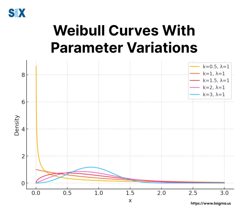
While the exponential model is simple, its constant hazard assumption is often too restrictive. The Weibull distribution is a far more flexible two-parameter model that is widely used in reliability and actuarial science. Its parameters are a scale parameter $λ > 0$ and a shape parameter $κ > 0$ .

Interpreting the Weibull Parameters

The true power of the Weibull distribution comes from the interpretation of its shape parameter, $κ$ :

$κ < 1$ : The hazard rate is decreasing over time. This models "infant mortality," where failures are more likely to occur early in the lifetime of a component or policy.
$κ = 1$ : The hazard rate is constant. The Weibull distribution simplifies to the exponential distribution with rate $λ$ .
$κ > 1$ : The hazard rate is increasing over time. This models failure due to wear-out or aging, where the risk of an event increases with time.

The scale parameter $λ$ acts similarly to the exponential rate, stretching or compressing the distribution on the time axis. The time $t = 1/ λ$ is known as the "characteristic life" of the distribution.

This plot shows several Weibull probability density functions. Notice how the shape parameter `k` (our $\kappa$) fundamentally alters the curve. For k=1, we get the familiar declining exponential shape. For k>1, the density has a distinct peak, indicating a "most likely" time of failure, which is characteristic of wear-out processes.

Finding the MLEs for the Weibull Distribution

The log-likelihood for the Weibull model is more complex, and differentiating it with respect to $λ$ and $κ$ results in a system of two non-linear equations. Unlike the exponential model, there is no simple closed-form solution. The MLEs must be found using numerical optimization algorithms like Newton-Raphson, which are implemented in all major statistical software packages.

For the CS2 exam, you are not expected to solve these equations by hand, but you must understand how they are derived and, most importantly, how to interpret the results.

Chapter 5: Statistical Methods in Survival Analysis

This section extends the MLE framework to the two-parameter Weibull model.

Please read the section on the Weibull Distribution. Your focus should be on: The structure of the log-likelihood function and the resulting score equations. Appreciate why a numerical solution is necessary. The ball bearing data example. Pay close attention to how the authors compare the Weibull fit to the exponential fit. Notice that \hat{\kappa} = 2.10, which is greater than 1. This provides strong evidence of an increasing hazard (wear-out), making physical sense for ball bearings and explaining why the exponential model was a poor fit. The use of the likelihood ratio statistic to formally test whether the Weibull model provides a significantly better fit than the exponential model. This is a critical skill for model comparison.

Model Selection and Interpretation

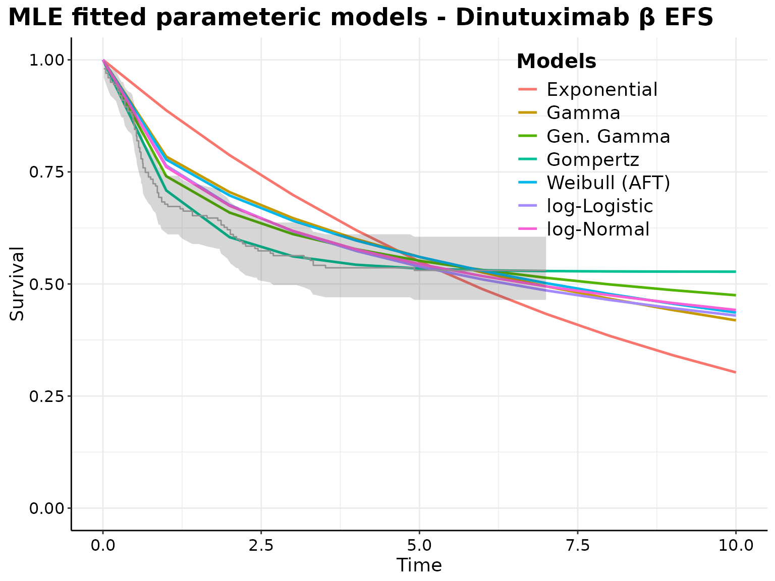
The ball bearing example highlights a crucial aspect of this topic: fitting a model is just the first step. The second, equally important step is interpretation and assessment. When we fit a Weibull model and find $κ^= 2.10$ , we have gained insight into the failure process itself.

A key tool for comparing a simpler model (e.g., Exponential) to a more complex, nested model (e.g., Weibull) is the Likelihood Ratio Test (LRT). Since the exponential is just a Weibull with $κ = 1$ , we can test the null hypothesis $H_{0} : κ = 1$ . The test statistic is:

LRT = 2 \times (l (λ^_{Weibull}, κ^_{Weibull}) - l (λ^_{Exp}))

Under the null hypothesis, this statistic follows a $χ^{2}$ distribution with degrees of freedom equal to the difference in the number of parameters (in this case, $2 - 1 = 1$ ).

For the ball bearing data, the log-likelihoods were -113.69 for the Weibull and -121.44 for the exponential.

LRT = 2 \times (- 113.69 - (- 121.44)) = 15.5

The critical value for a $χ_{1}^{2}$ test at the 5% significance level is 3.84. Since 15.5 is far greater than 3.84, we strongly reject the null hypothesis. We can conclude with high confidence that the Weibull model is a statistically significant improvement over the exponential model for this data, confirming that the assumption of a constant hazard rate is inappropriate.

As seen in the previous lesson, fitting multiple models allows for visual comparison. The LRT provides a formal statistical method to decide if a more complex model (like Weibull) is justified over a simpler one (like Exponential).

Conclusion

In this lesson, you have moved from formulating a likelihood function to actively using it to fit and interpret parametric survival models. This is a core competency for an actuary, combining probability theory with practical data analysis.

Key Takeaways:

Maximum Likelihood Estimation for survival models involves maximizing a log-likelihood function that correctly incorporates both event times and censored times.
The MLE for the exponential rate parameter $λ$ has an intuitive closed-form solution: $λ^= (Total Events) / (Total Time on Test)$ .
For multi-parameter models like the Weibull, MLEs are found using numerical methods, but the interpretation of the parameters (especially the shape parameter $κ$ ) provides deep insight into the nature of the risk.
The Likelihood Ratio Test is a powerful tool for statistically comparing nested models (e.g., Weibull vs. Exponential) to determine if increased model complexity is justified by the data.

So far, our models have assumed a single, homogeneous population. In our next module, we will explore the Cox Proportional Hazards Model, a powerful semi-parametric technique that allows us to model how covariates (like age, gender, or treatment group) influence survival, without making strong assumptions about the underlying shape of the hazard function.

Recommended resources