Introduction to Cox Proportional Hazards Model

Introduction

In our last lesson, we mastered fitting parametric survival models like the Exponential and Weibull distributions using maximum likelihood estimation. A key limitation of that approach is its reliance on a strong assumption: that the hazard function for the entire population follows a specific mathematical form. This is often too rigid for real-world actuarial data, where different individuals face different levels of risk based on their characteristics.

This lesson introduces a far more flexible and widely used technique: the Cox Proportional Hazards (PH) model. We will explore how this powerful semi-parametric model allows us to analyze the relationship between an individual's characteristics—or covariates—and their survival time. Your goal is to understand the structure of the Cox model and, most importantly, learn how to interpret its primary output: the regression coefficients. This skill is fundamental to modern survival analysis and a cornerstone of the CS2 syllabus.

Moving Beyond Homogeneous Populations

The models we've studied so far, such as the Weibull model, treat the population as a single, homogeneous group. The estimated parameters, like $λ$ and $κ$ , apply to everyone. But in practice, an actuary needs to answer questions like:

How does being a smoker affect a person's mortality risk compared to a non-smoker?
Do older policyholders have a higher lapse rate than younger ones?
Is a new medical treatment more effective than the standard one?

To answer these questions, we need a regression framework for survival data. The Cox model, developed by Sir David Cox in 1972, provides exactly this. Its brilliance lies in its ability to quantify the effect of covariates on risk without making any assumptions about the underlying shape of the hazard function over time.

Defining the Cox Proportional Hazards Model

The Cox model specifies that the hazard rate $λ (t)$ for an individual at time $t$ depends on a set of $p$ covariates $Z = (Z_{1}, Z_{2}, \dots, Z_{p})$ according to the following formula:

λ (t; Z) = λ_{0} (t) exp (β_{1} Z_{1} + β_{2} Z_{2} + \dots + β_{p} Z_{p})

Let's break down this crucial equation:

$λ (t; Z)$ is the hazard function for an individual with a specific set of covariate values $Z$ .
$λ_{0} (t)$ is the baseline hazard function. This is the non-parametric part of the model. It represents the hazard rate for a hypothetical individual for whom all covariates $Z_{j}$ are equal to zero. The model's key innovation is that we can estimate the $β$ coefficients without needing to know or assume the form of $λ_{0} (t)$ .
$exp (β_{1} Z_{1} + \dots + β_{p} Z_{p})$ is the parametric part. It's a linear combination of the covariates, transformed by the exponential function to ensure the resulting hazard is positive. The coefficients $β_{1}, \dots, β_{p}$ are the regression coefficients we estimate from the data.

For a deeper look at the model's mathematical structure, the following reading provides a formal definition.

[PDF] Modeling of Survival Data

This document from the University of Michigan provides a concise mathematical introduction to the Cox PH model.

Focus your reading on these two parts: The definition of the Cox model formula. The explanation of the Baseline Hazard Function and the general form with multiple covariates. Note how the model is framed as a linear model for the log of the hazard ratio.

The Proportional Hazards Assumption

The model gets its name from its central assumption: proportional hazards. This means that the ratio of the hazards for any two individuals is constant over time.

Consider two individuals, A and B, with different covariate vectors $Z_{A}$ and $Z_{B}$ . Their hazard ratio is:

\frac{λ ( t ; Z _{A} )}{λ ( t ; Z _{B} )} = \frac{λ _{0} ( t ) exp ( β ^{'} Z _{A} )}{λ _{0} ( t ) exp ( β ^{'} Z _{B} )} = exp (β^{'} (Z_{A} - Z_{B}))

Notice that the baseline hazard $λ_{0} (t)$ cancels out, leaving a value that depends only on the covariates and their coefficients, not on time $t$ . If individual A has twice the risk of an event as individual B at the beginning of the study, they are assumed to have twice the risk at any point in time.

The video below gives an excellent conceptual explanation of this assumption, drawing an analogy to the absence of an interaction effect in linear regression—a concept that will be familiar from your statistical background.

Survival Analysis Part 9 | Cox Proportional Hazards Model

This video from MarinStatsLectures provides a clear intuition for the proportional hazards assumption.

Watch the following segments: The introduction, which defines the core idea of a constant hazard ratio. The explanation of proportional hazards, which draws parallels to linear and logistic regression models that have no effect modification (interaction). The visual of parallel lines on a log-hazard scale is particularly insightful.

Interpreting Coefficients and Hazard Ratios

The primary goal of fitting a Cox model is to understand the relationship between the covariates and the risk of an event. This is done by interpreting the estimated coefficients, $β^_{j}$ .

Since the model is $λ (t; Z) = λ_{0} (t) exp (\sum β_{j} Z_{j})$ , we can rearrange it to see it as a linear model for the log-hazard ratio relative to the baseline:

lo g (\frac{λ ( t ; Z )}{λ _{0} ( t )}) = β_{1} Z_{1} + β_{2} Z_{2} + \dots + β_{p} Z_{p}

From this, we can see that a $β_{j}$ coefficient represents the change in the log-hazard for a one-unit increase in the corresponding covariate $Z_{j}$ , holding all other covariates constant.

While this is technically correct, it's not very intuitive. A much more direct interpretation is achieved by exponentiating the coefficient to get the Hazard Ratio (HR).

The Hazard Ratio (HR)

The hazard ratio for a covariate $Z_{j}$ is $HR_{j} = exp (β_{j})$ . It represents the multiplicative effect on the hazard rate for a one-unit increase in $Z_{j}$ .

The rules for interpretation are straightforward:

If $β_{j} > 0$ , then $HR_{j} > 1$ . An increase in $Z_{j}$ is associated with an increased hazard of the event.
If $β_{j} < 0$ , then $HR_{j} < 1$ . An increase in $Z_{j}$ is associated with a decreased hazard (a protective effect).
If $β_{j} = 0$ , then $HR_{j} = 1$ . The covariate $Z_{j}$ has no effect on the hazard.

For example, if a covariate "smoker" (coded as 1 for smokers, 0 for non-smokers) has a coefficient $β^= 0.693$ , the hazard ratio is $exp (0.693) \approx 2.0$ . We would interpret this as: "Smokers have twice the hazard of death compared to non-smokers, after controlling for other factors in the model."

If a drug treatment (coded 1 for treated, 0 for placebo) has a coefficient $β^= - 0.51$ , the HR is $exp (- 0.51) \approx 0.60$ . The interpretation: "The group receiving the treatment has a 40% lower hazard of death (since $1 - 0.60 = 0.40$ ) compared to the placebo group."

The following video provides an excellent, detailed walkthrough of interpreting both coefficients and hazard ratios from a typical model output.

COX REGRESSION and HAZARD RATIOS - easily explained with an example!

This Biostatsquid video explains how to interpret the outputs of a Cox regression model with a clear clinical example.

Please watch these two key sections: Coefficients and Hazard Ratios: This part explains the relationship between the log-hazard-ratio (coefficient) and the hazard ratio, and how to interpret each. A Worked Example: This demonstrates the interpretation of a full model with multiple covariates (treatment, age, gender), including how to consider statistical significance (p-values) and confidence intervals.

Visualizing Hazard Ratios

A common way to present the results of a Cox model is with a forest plot, which visualizes the hazard ratios and their confidence intervals for multiple covariates simultaneously.

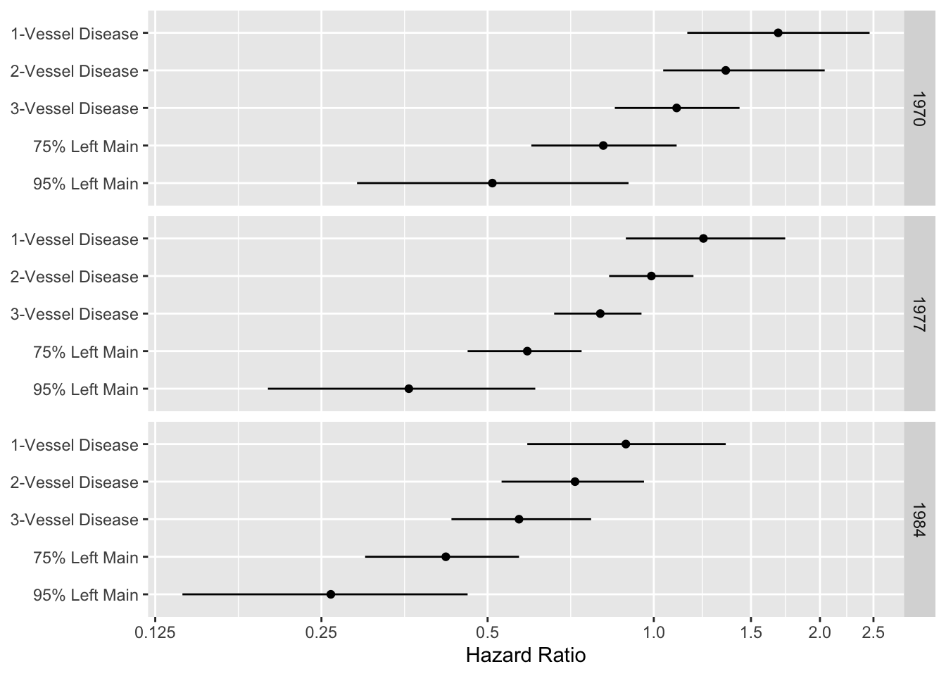
This plot shows estimated hazard ratios from a study comparing coronary artery bypass graft (CABG) surgery to medical therapy for patients with varying degrees of heart disease. The x-axis is the Hazard Ratio. The reference group is patients receiving medical therapy, so a hazard ratio less than 1 indicates that surgery is more beneficial (lower hazard of death). A hazard ratio greater than 1 would suggest surgery is riskier. The horizontal lines are 95% confidence intervals. If a confidence interval does not cross the vertical line at HR=1.0, the result is statistically significant.

Let's interpret one line from the 1984 data:

95% Left Main: The dot is at approximately HR = 0.25. This means that for patients with severe (95%) blockage of the left main artery, undergoing surgery reduces their hazard of death by about 75% compared to receiving only medical therapy. The confidence interval is entirely below 1.0, indicating this is a highly significant protective effect.
1-Vessel Disease: The dot is around HR = 1.1, and the confidence interval clearly crosses 1.0. This suggests there is no statistically significant difference in hazard between surgery and medical therapy for patients with less severe disease.

This plot elegantly summarizes the model's findings: surgery provides a substantial survival benefit for patients with severe disease, but its benefit diminishes and may not exist for those with milder disease.

Conclusion

In this lesson, we have laid the theoretical groundwork for one of the most important tools in the actuary's toolkit. You have learned that the Cox model provides a robust method for understanding how different risk factors affect survival, without needing to make restrictive assumptions about the baseline hazard.

Key Takeaways:

The Cox Proportional Hazards model has the form $λ (t; Z) = λ_{0} (t) exp (β^{'} Z)$ , separating a non-parametric baseline hazard from a parametric component based on covariates.
Its core assumption is that the ratio of hazards between any two individuals is constant over time.
The regression coefficient $β_{j}$ represents the change in the log-hazard for a one-unit increase in the covariate $Z_{j}$ .
The Hazard Ratio, $HR_{j} = exp (β_{j})$ , is the most intuitive output. It quantifies the multiplicative factor by which the hazard changes for a one-unit increase in the covariate. A HR > 1 means increased risk, and a HR < 1 means decreased risk.

We have focused on what the model is and how to interpret its results. In our next lesson, we will address the crucial question of how we estimate the $β$ coefficients. This will lead us to the ingenious concept of partial likelihood, a key theoretical component you'll need for the exam.

Recommended resources