Likelihood for Censored Survival Data

Introduction

Welcome to our next lesson. In the previous part of this module, we explored non-parametric methods for survival analysis, culminating in the log-rank test for comparing survival curves. While powerful for testing hypotheses, non-parametric methods don't assume an underlying shape for the survival distribution, which means they can't be used to model the survival function with a specific mathematical formula or to easily predict survival at times beyond the observed data.

Today, we pivot to parametric survival modeling. This approach involves assuming that the time-to-event data follows a specific probability distribution (like the Exponential, Weibull, or Gompertz distribution). Our goal in this lesson is to tackle the foundational step for any parametric estimation: learning to formulate the likelihood function for a parametric survival model with censored data.

As a statistician, you are well-acquainted with the principle of maximum likelihood. The core challenge in survival analysis is constructing a likelihood function that correctly accounts for the incomplete information provided by censored observations. Mastering this will directly prepare you for our next lesson, where we will maximize these functions to estimate model parameters.

From Observations to Likelihood: Handling Censored Data

In survival analysis, not all data points are created equal. We have exact event times, but we also have censored observations where the event has not yet occurred or was otherwise not observed. Before we can write down a mathematical expression for likelihood, we must be clear about what information each type of observation provides.

This diagram illustrates the common types of observations in a survival study. An individual has an event (1, 4), is right-censored (2, 3), or is interval-censored (5). Our likelihood function must correctly represent the information from each case.

The key principle is that the likelihood of the entire dataset is the product of the probabilities of each individual observation, assuming they are independent. The contribution of each individual to this product depends on whether their event time was observed or censored:

Exact Event: If an individual has an event at time $t$ , their contribution is the probability density of the event occurring at that exact moment, given by the probability density function, $f (t)$ .
Right-Censored: If an individual is censored at time $t$ , we only know that their true event time is greater than $t$ . Their contribution is the probability of this, which is the survival function, $S (t)$ .
Left-Censored: If an individual is censored at time $t$ , we know their event occurred before $t$ . The probability is $P (T < t)$ , which is the cumulative distribution function, $F (t) = 1 - S (t)$ .
Interval-Censored: If we only know the event occurred between times $L$ and $R$ , the probability is $P (L < T < R) = S (L) - S (R)$ .

The following reading provides a clear, step-by-step development of how each of these observation types contributes to the total likelihood function.

[PDF] Likelihood construction - MyWeb

This document by Patrick Breheny from the University of Iowa gives an excellent formal introduction to constructing likelihoods for censored and truncated data.

Begin by reading the introductory slides on the definition of likelihood for continuous distributions. Then, follow the logic for fully observed data. The core of your reading should focus on the sections explaining the likelihood contributions for right censoring, left censoring, and interval censoring. Finally, study the summary table at the end, which provides a concise and valuable reference for each case.

The General Likelihood Function for Right-Censored Data

Right-censoring is the most common scenario in survival analysis. To handle it efficiently, we typically represent our data for each individual $i$ as a pair: $(y_{i}, δ_{i})$ , where:

$y_{i}$ is the observed time, which is either the time of event or the time of censoring.
$δ_{i}$ is an event indicator: $δ_{i} = 1$ if an event occurred at time $y_{i}$ , and $δ_{i} = 0$ if the observation was right-censored at time $y_{i}$ .

Using this notation, we can write a single, elegant expression for the contribution of any individual to the likelihood. The contribution for individual $i$ is:
$L_{i} (θ) = [f (y_{i} ∣ θ)]^{δ_{i}} [S (y_{i} ∣ θ)]^{1 - δ_{i}}$
Here, $θ$ represents the vector of parameters for our chosen parametric model (e.g., $θ = λ$ for an exponential model).

If $δ_{i} = 1$ (an event), the expression becomes $f (y_{i} ∣ θ)$ . If $δ_{i} = 0$ (censored), it becomes $S (y_{i} ∣ θ)$ . The total likelihood for a sample of $n$ individuals is the product of these individual contributions:
$L (θ) = \prod_{i = 1}^{n} [f (y_{i} ∣ θ)]^{δ_{i}} [S (y_{i} ∣ θ)]^{1 - δ_{i}}$

Since the hazard function $h (t)$ and survival function $S (t)$ are related to the density function by $f (t) = h (t) S (t)$ , we can substitute this into the likelihood expression:
$L (θ) = \prod_{i = 1}^{n} [h (y_{i} ∣ θ) S (y_{i} ∣ θ)]^{δ_{i}} [S (y_{i} ∣ θ)]^{1 - δ_{i}} = \prod_{i = 1}^{n} [h (y_{i} ∣ θ)]^{δ_{i}} S (y_{i} ∣ θ)$
This form is especially useful for models defined by their hazard rate.

The next reading will walk you through this formalization and provide concrete examples.

[PDF] STAT574/STAT474: Survival - Department of Mathematics & Statistics

These lecture notes from the University of New Mexico provide a clear derivation of the general likelihood function for right-censored data.

Please read the section titled "The likelihood with right-censoring". Focus on how the general expression L = \prod [f(t_i)]^{\delta_i}[S(t_i)]^{1-\delta_i} is constructed and then re-expressed in terms of the hazard function.

Worked Example: The Exponential Distribution

Let's apply this framework to a tangible case. Suppose we assume our survival times follow an Exponential distribution with rate parameter $λ$ . The key functions are:

PDF: $f (t ∣ λ) = λ e^{- λ t}$
Survival function: $S (t ∣ λ) = e^{- λ t}$

Plugging these into our general likelihood formula gives:

L (λ) = i = 1 \prod n [λ e^{- λ y_{i}}]^{δ_{i}} [e^{- λ y_{i}}]^{1 - δ_{i}}

We can simplify this by combining the exponents:

L (λ) = i = 1 \prod n λ^{δ_{i}} e^{- λ y_{i} δ_{i}} e^{- λ y_{i} (1 - δ_{i})} = i = 1 \prod n λ^{δ_{i}} e^{- λ y_{i}}

Let $d = \sum_{i = 1}^{n} δ_{i}$ be the total number of observed events. The likelihood simplifies to:

L (λ) = λ^{d} exp (- λ i = 1 \sum n y_{i})

In practice, it is almost always easier to work with the log-likelihood, as it turns the product into a sum:

ln L (λ) = l (λ) = d ln (λ) - λ i = 1 \sum n y_{i}

This is the function we would maximize in our next lesson to find the maximum likelihood estimate (MLE) for $λ$ .

Now, let's see how this is applied to a numeric example and then see the setup for a more complex, two-parameter distribution.

[PDF] STAT574/STAT474: Survival - Department of Mathematics & Statistics

This resource continues with excellent, practical examples.

First, carefully review the Exponential distribution example. Note how the formula we just derived is used with actual data. Then, read through the setup for the log-logistic example. You don't need to follow all the algebraic simplification, but focus on how the likelihood is constructed as a product of terms for events (f(x)) and, in this case, left-censored observations (1-S(x)).

The process for the log-logistic model, or any other parametric model like the Weibull, Gompertz, or log-normal, is identical in principle:

Choose a parametric distribution.
Write down its density $f (t ∣ θ)$ and survival $S (t ∣ θ)$ functions.
For each observation in your dataset, select the appropriate term ( $f (t)$ for events, $S (t)$ for right-censoring, etc.).
The total likelihood is the product of these terms.

The result is a function of the model parameters $θ$ which represents the likelihood of observing your specific dataset.

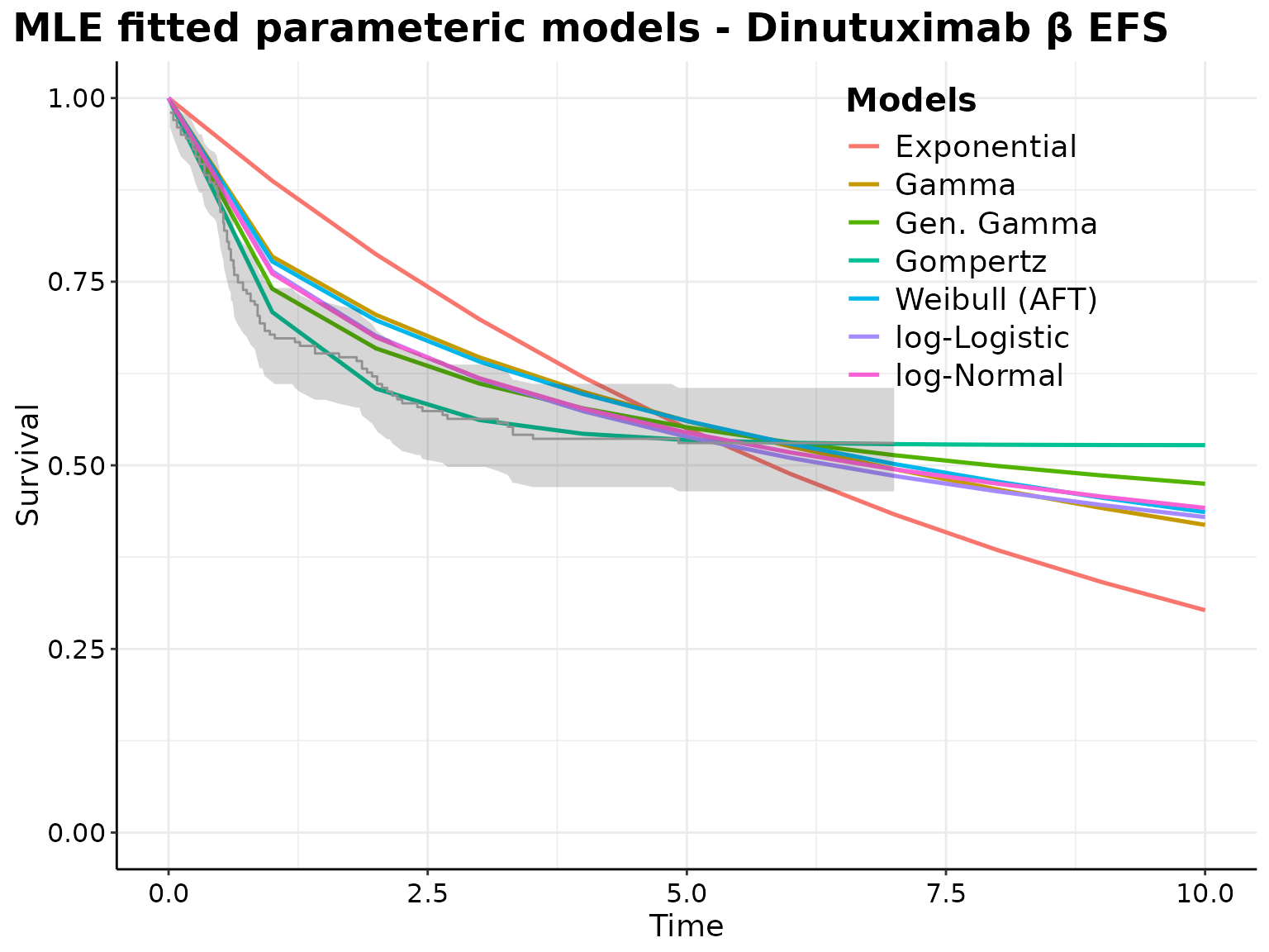
Once a likelihood function is formulated for a chosen parametric model (e.g., Exponential, Weibull, Gompertz), it can be maximized to find the best-fitting parameters. This plot shows the survival curves resulting from fitting several different parametric models to the same dataset, an outcome of the process we'll cover in the next lesson.

Conclusion

In this lesson, we established the crucial methodology for parametric survival modeling: constructing the likelihood function from censored data. You learned that the key is to ensure each observation contributes to the likelihood in a way that reflects the information it contains.

Key Takeaways:

The likelihood function for survival data is a product of terms, where each term represents the probability of an individual observation.
Events contribute the probability density function, $f (t)$ .
Right-censored observations contribute the survival function, $S (t)$ .
Left-censored observations contribute the CDF, $F (t)$ .
For a dataset with events and right-censoring, the likelihood can be compactly written as $L (θ) = \prod [f (y_{i})]^{δ_{i}} [S (y_{i})]^{1 - δ_{i}}$ .

We have now laid all the necessary groundwork. In our next lesson, we will put this knowledge into practice by fitting parametric survival models using maximum likelihood estimation (MLE) and learning how to interpret the resulting parameters.

Recommended resources

Introduction

From Observations to Likelihood: Handling Censored Data

The General Likelihood Function for Right-Censored Data

Worked Example: The Exponential Distribution

Conclusion