Mortality Projection Models: A Comparative Analysis

The General Age-Period-Cohort (APC) Framework

Most modern stochastic mortality models can be understood as variations of a generalized structure that decomposes mortality rates by age, period (calendar year), and cohort (year of birth). Understanding this common framework is invaluable as it allows you to see the connections and key differences between seemingly disparate models.

A paper by Andrew Hunt and David Blake provides an excellent, holistic analysis of this structure.

As you've just read, the APC framework gives us a language to describe and compare models. A model is defined by its choices for:

• Response Variable & Link Function: E.g., $\ln ({\mu }_{x,t})$ or $\text{logit}(q_{x,t})$.
• Static Age Component (${\alpha }_x$): Captures the average shape of the mortality curve.
• Age/Period Terms (${\beta }_x^{(i)}{\kappa }_t^{(i)}$): Capture dynamic changes over time. The form of ${\beta }_x$ is a key differentiator.
  • Non-parametric: ${\beta }_x$ is estimated freely from the data for each age (like in the Lee-Carter model). This is flexible but uses many parameters.
  • Parametric: ${\beta }_x$ has a pre-defined algebraic form, like $1$, $(x-\bar{x})$, or $(x-\bar{x}{)}^2$. This is more parsimonious but less flexible.
• Age/Cohort Term (${\beta }_x^{(0)}{\gamma }_{t-x}$): Captures effects specific to generations born in the same year.

The original Lee-Carter model, $\ln ({\mu }_{x,t})={\alpha }_x+{\beta }_x{\kappa }_t$, is a simple APC model with one non-parametric age/period term and no cohort term.

Limitations and Extensions of the Lee-Carter Model

The original Lee-Carter model was groundbreaking, but practice revealed limitations. Ronald Lee, one of its creators, discusses some of these in the video below.

These limitations have inspired a range of "hybrid" models that extend the basic Lee-Carter structure within the APC framework. Let's look at the most common ones.

Let's summarize the key extensions:

• LC2 Model: $\ln ({\mu }_{x,t})={\alpha }_x+{\beta }_x^{(1)}{\kappa }_t^{(1)}+{\beta }_x^{(2)}{\kappa }_t^{(2)}$. This adds a second age/period interaction. It can capture more complex dynamics than the single-factor LC model, but the second component can be difficult to interpret demographically and challenging to forecast.
• Classic APC Model: $\ln ({\mu }_{x,t})={\alpha }_x+{\kappa }_t+{\gamma }_{t-x}$. This model is conceptually appealing due to its symmetry but suffers from a well-known identifiability problem: you can add a linear trend to the period effect and subtract it from the cohort effect without changing the model fit. Since you have a strong background in statistics, you can recognize this as a perfect collinearity issue.
• Renshaw-Haberman (RH) / H1 Model: $\ln ({\mu }_{x,t})={\alpha }_x+{\beta }_x{\kappa }_t+{\gamma }_{t-x}$. This is arguably the most important extension. By adding a simple cohort term (${\gamma }_{t-x}$) to the Lee-Carter structure, it directly addresses one of the original model's main weaknesses. It can capture persistent mortality differences between generations.

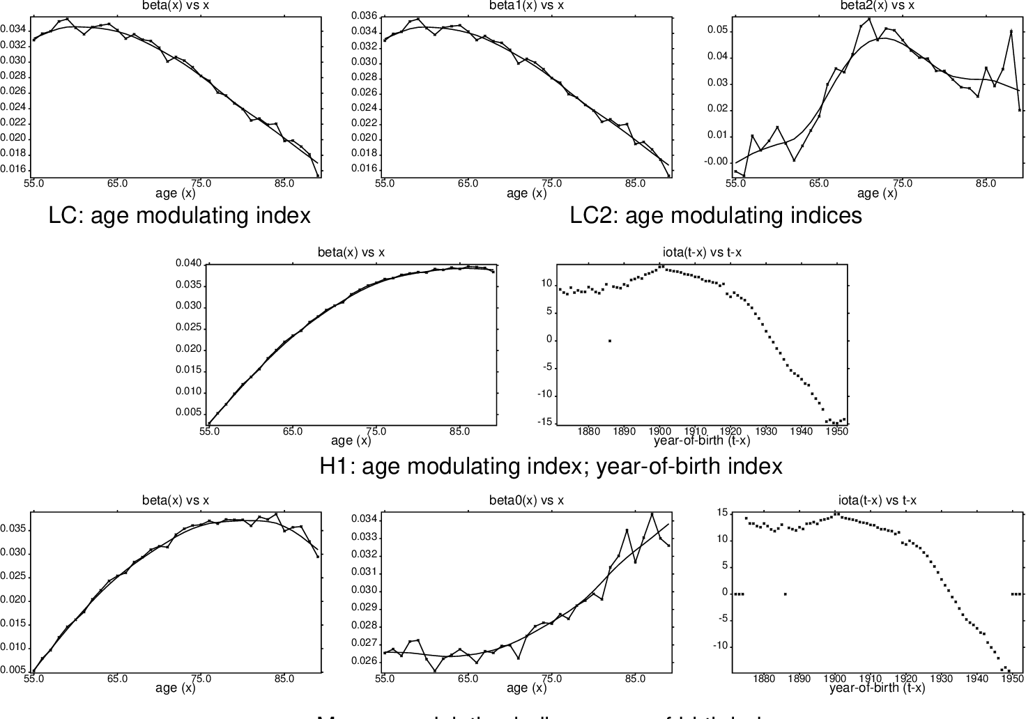
The image below shows the estimated parameters for several of these models. Notice how the models with a cohort term (H1, M) explicitly separate out a year-of-birth effect ($\iota (t-x)$), which is absent in the LC and LC2 models.

The Cairns-Blake-Dowd (CBD) Family

While the Lee-Carter family of models was developing, a parallel family of models emerged, specifically designed for modeling mortality at older ages, a key concern for pension funds and annuity providers. This is the Cairns-Blake-Dowd (CBD) family.

The key distinctions of the CBD model, $\text{logit}(q_{x,t})={\kappa }_t^{(1)}+(x-\bar{x}){\kappa }_t^{(2)}$, compared to Lee-Carter are:

1. Response Variable and Link: It models the one-year probability of death, $q_{x,t}$, using a logit link function, which is the canonical link for a binomial model of death counts. This is statistically elegant.
2. Age Functions: It uses parametric age functions. In the original model, ${\beta }_x^{(1)}=1$ and ${\beta }_x^{(2)}=(x-\bar{x})$. This assumes mortality improvements change linearly with age, which can be a reasonable approximation at older ages but is less suitable for the full age range.
3. Parsimony: By using pre-defined parametric age functions and omitting the static ${\alpha }_x$ term, the model is extremely parsimonious (has very few parameters). This is an advantage for smaller datasets, like those for a specific pension plan.

The extensions M6, M7, and M8 build on this by adding cohort terms and higher-order polynomial age effects, creating a family of models well-suited for annuity-related work.

A Data-Driven Alternative: P-Spline Models

Both the Lee-Carter and CBD families impose a fair amount of structure on the data. An alternative approach, rooted in non-parametric statistics, is to use P-splines (penalized splines). Instead of specifying a rigid structure, this method aims to fit a smooth surface to the observed mortality rates across age and time.

The core idea of P-splines is to balance two competing goals:

• Goodness-of-Fit: You want the model to fit the historical data well. This is achieved by using a large number of flexible basis functions (B-splines).
• Smoothness: You want to avoid overfitting and produce a biologically plausible, smooth mortality surface. This is achieved by adding a penalty to the likelihood function that punishes "wiggliness" or lack of smoothness in the fitted surface.

From a statistical perspective, you can think of this as a form of penalized regression. The main advantage is flexibility. A P-spline model doesn't assume a fixed age pattern of improvement. It lets the data reveal the patterns, including cohort effects and rotation, which emerge naturally from the fitted surface. The main disadvantage is that it can be more of a "black box," with less direct demographic interpretation of its components compared to an APC model.

Model Comparison and Selection

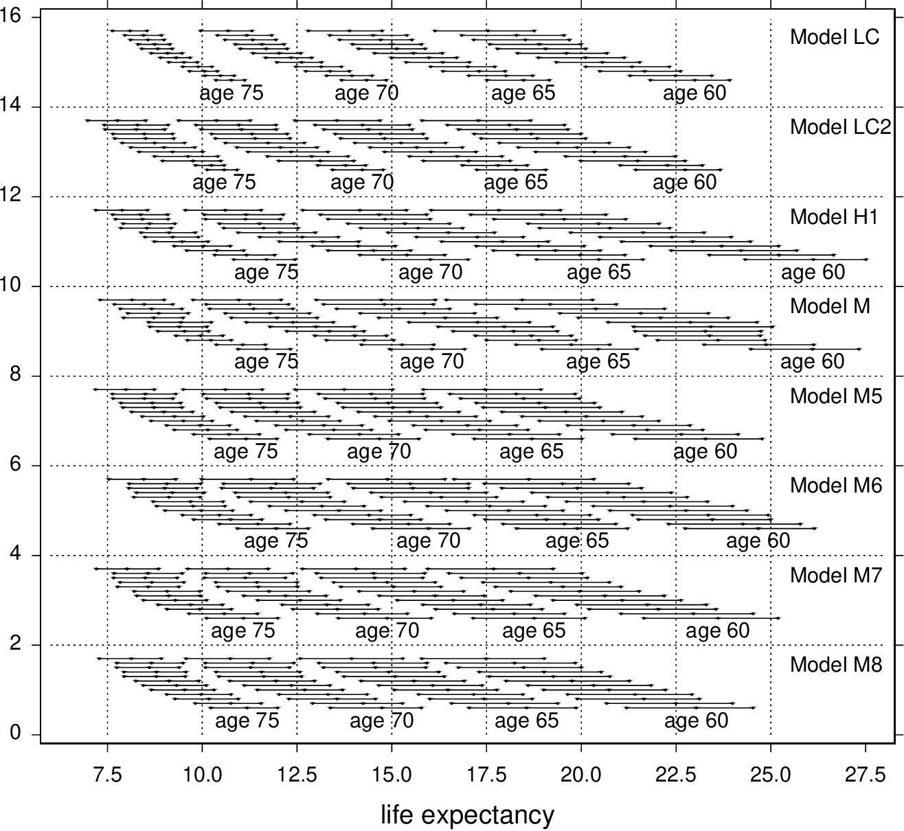
We have now surveyed a landscape of models. There is no single "best" model for all situations. The choice depends on the specific goals, data, and desired trade-offs. The image below shows how different models can produce different central forecasts and levels of uncertainty for life expectancy.

The paper "On the Structure and Classification of Mortality Models" concludes with five key principles for selecting or constructing a model, which serve as an excellent summary for a practicing actuary.

The essential trade-off is often between demographic interpretability and statistical flexibility.

• Lee-Carter and CBD models have clear, interpretable components (${\kappa }_t$ as a general trend, ${\gamma }_{t-x}$ as a cohort effect) but impose a rigid structure.
• P-spline models are highly flexible and can capture complex patterns but lack the simple, separable components of APC models.

Conclusion

In this lesson, we have expanded our view beyond the Lee-Carter model to appreciate the rich variety of tools available for mortality projection. We have seen that most popular models can be understood within a unifying Age-Period-Cohort framework, and their differences can be analyzed through their choices of link function, age functions, and inclusion of cohort effects.

Key Takeaways:

• APC Framework: This general structure (${\eta }_{x,t}={\alpha }_x+\sum {\beta }_x^{(i)}{\kappa }_t^{(i)}+{\beta }_x^{(0)}{\gamma }_{t-x}$) is a powerful tool for classifying and understanding models.
• Lee-Carter Family: The original LC model can be extended with additional period terms (LC2) or, more importantly, with a cohort term (RH model) to capture generational effects. These models typically use non-parametric age functions.
• CBD Family: These models use a logit link and parametric (e.g., linear) age functions, making them parsimonious and well-suited for older-age mortality, as found in annuity portfolios.
• P-Spline Models: This is a flexible, data-driven smoothing approach that balances goodness-of-fit with smoothness. It can capture complex patterns like rotation and cohort effects without them being explicitly defined in the model formula.
• Model Selection: There is no universally superior model. The choice involves a trade-off between interpretability, flexibility, and parsimony, and should be guided by the purpose of the analysis and the characteristics of the data.

Preview of the Next Module

This lesson concludes our module on projecting mortality over time. We have focused on modeling the timing of death. In our next module, Modeling Insurance Losses, we will shift our focus to an entirely different dimension of risk: the size of financial losses when an insured event occurs. We will begin by exploring how to fit standard probability distributions to data on insurance claim severities, a foundational skill in property, casualty, and health insurance.