Maximum Likelihood Estimation for Loss Distributions

Why Fit Distributions to Data?

When an insurer receives a set of historical claim data, it is simply a list of numbers. To make this data useful for predicting future costs, we need to generalize it by fitting a continuous probability distribution. A fitted model is easier to work with than raw data and allows us to answer crucial questions, such as:

• What is the expected cost of the next claim?
• What is the probability that a claim will exceed a very high threshold, like $1 million?
• How much capital should be held to cover potential losses with 99.5% confidence?

The overall process of fitting a model to loss data involves several steps, from exploring the data to selecting a model and estimating its parameters.

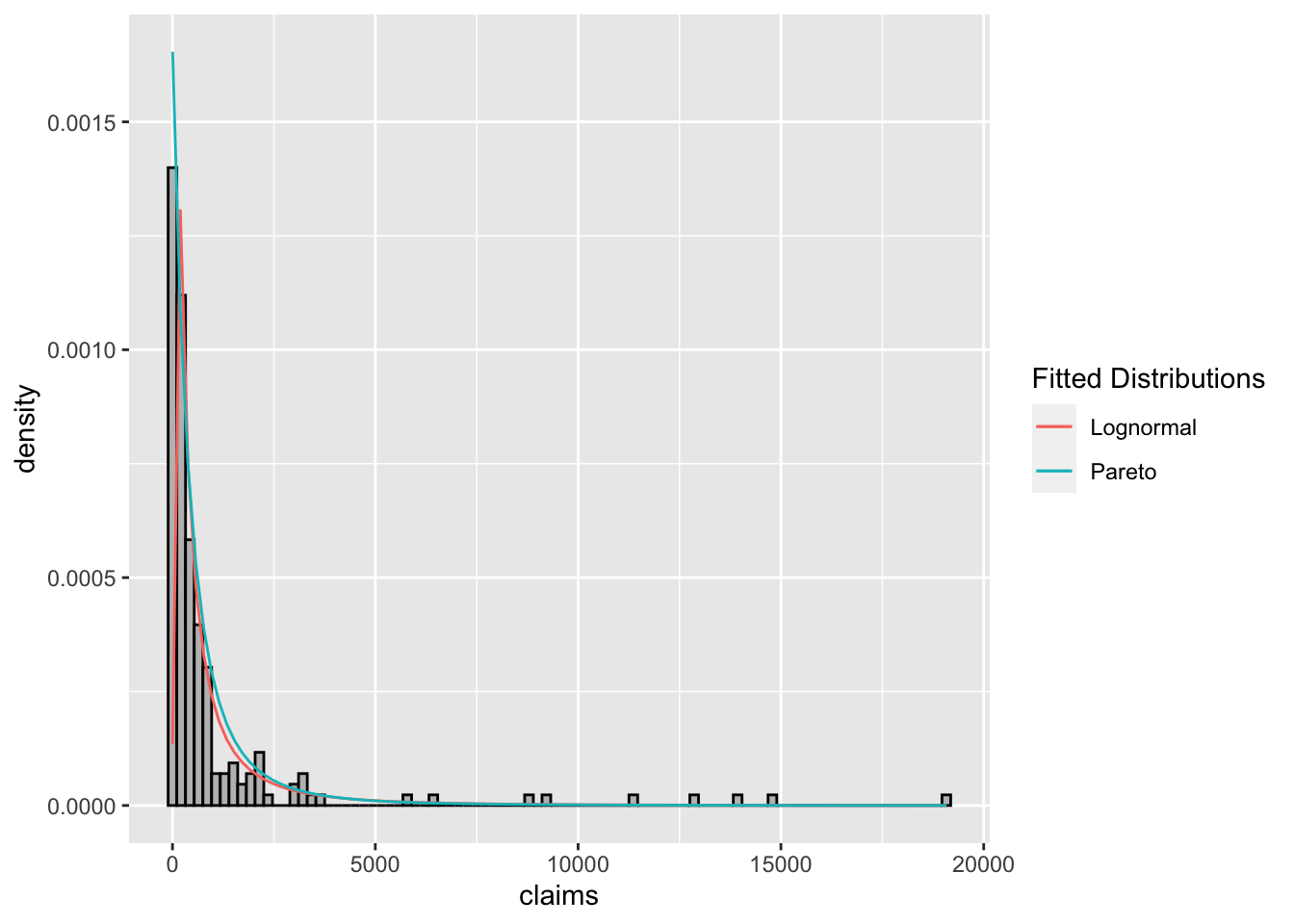
The image below illustrates the end product of this process. The histogram shows the empirical distribution of a set of insurance claims, and the colored lines represent two different parametric distributions (Lognormal and Pareto) that have been fitted to this data. Our goal today is to understand how to find the "best fitting" line.

The Intuition of Maximum Likelihood Estimation

So, what does it mean for a model to be the "best fit"? The principle of maximum likelihood provides a powerful and intuitive answer: The best model parameters are those that maximize the probability (or "likelihood") of having observed the actual data.

Imagine you have a handful of data points and a distribution, say a normal distribution. You can slide the distribution left and right (changing its mean) and make it wider or narrower (changing its standard deviation). For each combination of mean and standard deviation, you can calculate the collective probability of your data points under that specific version of the distribution. MLE simply finds the exact combination of parameters that makes this probability as high as possible.

The following video from StatQuest provides an excellent visual explanation of this core concept.

The Mechanics of Maximum Likelihood Estimation

Now, let's formalize the intuition from the video using calculus.

Suppose we have a random sample of $n$ independent and identically distributed observations $x_1,x_2,\dots ,x_n$. We assume these observations come from a probability density function (PDF) $f(x;\mathbf{\theta })$, where $\mathbf{\theta }$ is the vector of parameters we want to estimate.

Because the observations are independent, their joint probability density is the product of their individual densities. This joint density, viewed as a function of the parameters $\mathbf{\theta }$ given the fixed data, is called the likelihood function:

Our goal is to find the value of $\mathbf{\theta }$ that maximizes $L(\mathbf{\theta })$.

For both analytical and numerical reasons, it is almost always easier to work with the natural logarithm of the likelihood function, known as the log-likelihood function, $l(\mathbf{\theta })$. Since the logarithm is a strictly increasing function, maximizing $l(\mathbf{\theta })$ is equivalent to maximizing $L(\mathbf{\theta })$.

The log-likelihood handily converts the product into a sum, which is much easier to differentiate.

The general procedure to find the Maximum Likelihood Estimator(s), $\hat{\mathbf{\theta }}$, is:

1. Write down the log-likelihood function $l(\mathbf{\theta })$.
2. Take the partial derivative of $l(\mathbf{\theta })$ with respect to each parameter in $\mathbf{\theta }$.
3. Set these derivatives equal to zero. This gives a system of equations known as the likelihood equations.
4. Solve the likelihood equations for the parameters. The solution is the MLE, $\hat{\mathbf{\theta }}$.
5. (Optional but good practice) Verify that this solution corresponds to a maximum by checking that the matrix of second partial derivatives (the Hessian matrix) is negative definite at $\hat{\mathbf{\theta }}$.

Let's see this entire process in action for the exponential distribution, a common model for insurance losses.

MLE for Common Loss Distributions

Now that we have established the general procedure, let's apply it to a couple of other distributions that are mainstays in actuarial modeling: the Lognormal and Pareto distributions.

The Lognormal distribution is often used for claim amounts because it is positive-valued and skewed to the right. A random variable $X$ is lognormally distributed if $\ln (X)$ is normally distributed.

The Pareto distribution is particularly important for modeling large losses. It is a "heavy-tailed" distribution, meaning it assigns a higher probability to extreme events than distributions like the normal or exponential. This makes it suitable for modeling high-risk insurance claims and catastrophe losses.

The following reading walks through the MLE derivations for these distributions, framed as typical exam questions.

Conclusion

In this lesson, we have established the foundational technique for fitting severity models in insurance. We moved from the high-level intuition of finding the "best fit" to the concrete calculus of maximizing a likelihood function.

Key Takeaways:

• Objective: We fit parametric distributions to loss data to generalize from historical observations and create a predictive model for claim severity.
• Maximum Likelihood Principle: The core idea is to find the parameter values that make our observed data the most probable.
• Log-Likelihood: In practice, we maximize the log-likelihood function, which is analytically more convenient and numerically more stable than the likelihood function itself.
• Procedure: The process involves setting up the log-likelihood function, differentiating with respect to the parameters, setting the derivatives to zero, and solving the resulting likelihood equations.
• Common Estimators: We saw that this procedure leads to well-known estimators. For instance, the MLE for the exponential scale parameter is the sample mean, and the MLEs for the lognormal parameters $\mu$ and ${\sigma }^2$ are the sample mean and variance of the log-transformed data.

In this lesson, we have assumed that our data is "complete"—that is, every claim amount is recorded precisely. However, real-world insurance data is rarely so clean. Policies often include deductibles, which prevent us from observing small claims, and policy limits, which obscure the true size of very large claims.

Preview of the Next Lesson

Our next lesson will build directly on today's foundation. We will learn how to adapt the maximum likelihood framework to handle these common data features. You will learn how to construct the appropriate likelihood function for data that is truncated (due to deductibles) and censored (due to policy limits), a crucial skill for any practicing actuary.