Modeling Truncated and Censored Loss Data

What are Censoring and Truncation?

At a high level, both censoring and truncation deal with missing information, but they do so in fundamentally different ways.

• Censoring: We know an event (like a loss) has occurred and is part of our dataset, but we only have partial information about its value. For example, we might know the loss was "greater than $1 million" but not the exact amount. The observation is included, but its value is imprecise.
• Truncation: The event is not even recorded or observed if its value falls into a certain range. For example, claims below a $500 deductible might never be reported to the insurer, so they are entirely absent from the dataset. The observation is excluded.

The following video provides an excellent intuitive overview of the different types of censoring and truncation, using practical examples from survival analysis, which share the same underlying data structures as loss modeling.

To summarize the key ideas and connect them directly to insurance:

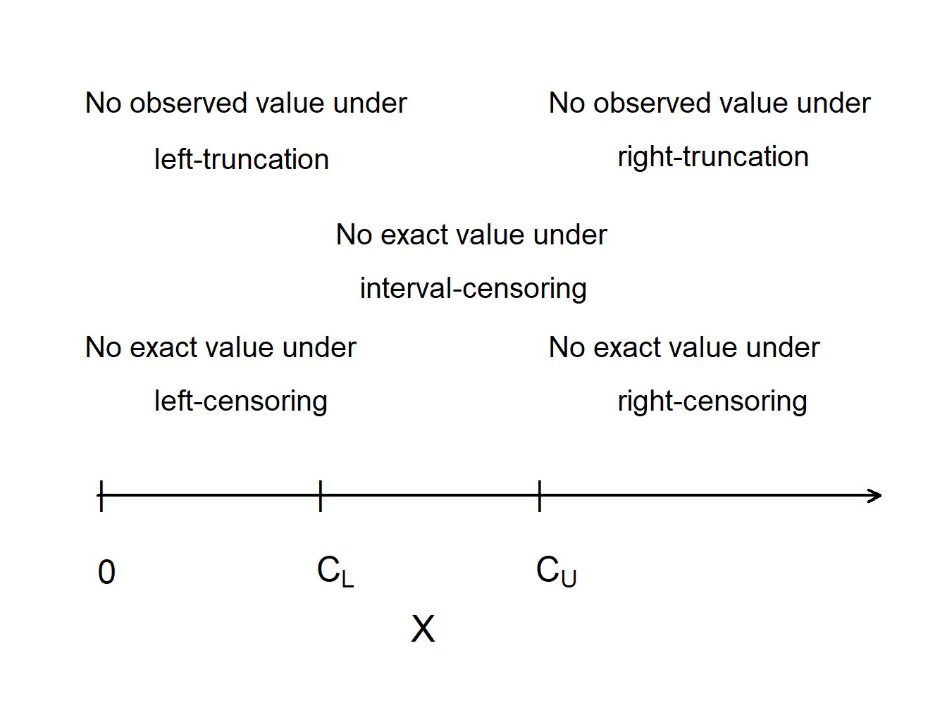
• Right-Censoring: This is the most common type in loss modeling. It occurs due to policy limits. If a policy has a limit of $u$, any loss greater than $u$ results in a payment of $u$. We record the value $u$, but we only know the true loss was at least $u$.
• Left-Truncation: This typically arises from deductibles. If a policy has a deductible $d$, losses smaller than $d$ are often not reported. Therefore, the insurer's data set is truncated from the left at $d$—it consists only of losses that were large enough to be reported.
• Left-Censoring: This occurs when we know a loss is below a certain threshold but don't know the exact value. In the context of deductibles, if an insurer records all losses, but only pays out the amount exceeding the deductible, the payment variable for a loss $X\le d$ is 0. This variable, $(X-d{)}_{+}=\max (0,X-d)$, is considered a left-censored and shifted variable.
• Interval-Censoring: This can happen if claims are only reviewed periodically. For example, if damages are assessed monthly, we might only know that a loss occurred sometime between two inspection dates.

The image below provides a simple visual summary of these concepts on a number line, where $X$ is the true, unobserved loss value.

Adjusting the Likelihood Function

Now for the crucial part: how do these data features change the likelihood function we learned about in the last lesson? The key is to represent the contribution of each data point based on what we actually know about it.

Let $f(x)$ be the PDF and $S(x)$ be the survival function of the loss distribution with parameters $\mathbf{\theta }$.

Contribution from Right-Censored Data

A policy limit is a classic source of right-censoring. If we observe a claim payment that hits the policy limit $u$, we don't know the true loss amount $x$, only that $x>u$. The probability of this event is $S(u)$.

So, for a dataset with $r$ exact observations $x_1,\dots ,x_r$ and $m$ observations right-censored at $u$, the likelihood function is:

Notice how the $m$ censored observations contribute $S(u)$ to the likelihood, not $f(u)$.

Contribution from Left-Truncated Data

A deductible is the most common cause of left-truncation. When data is left-truncated at a deductible $d$, our dataset only contains losses $x_i$ where $x_i>d$. Any likelihood calculation must be conditioned on this fact.

The probability density of observing a loss $x$, given that it was large enough to be included in our dataset (i.e., $X>d$), is a conditional density:

Therefore, for a dataset of $k$ observations $x_1,\dots ,x_k$, all of which are known to be greater than a deductible $d$, the likelihood function is:

The General Likelihood for Truncated and Censored Data

In many real-world insurance portfolios, policies have both a deductible (left-truncation) and a limit (right-censoring). We need a general likelihood function that can handle both simultaneously, and can even accommodate different deductibles and limits for different policies.

Let's represent each observation $j$ in our dataset by a triplet $(t_j,x_j,{\delta }_j)$, where:

• $t_j$ is the left-truncation point (the deductible).
• $x_j$ is the observed loss amount. For a censored observation, this is the policy limit.
• ${\delta }_j$ is a censoring indicator: ${\delta }_j=0$ for an exact observation, and ${\delta }_j=1$ for a right-censored observation.

The contribution of each data point to the likelihood is always conditional on the loss being greater than its truncation point $t_j$.

• If the observation is exact (${\delta }_j=0$): Its contribution is the conditional density $\frac{f(x_j)}{S(t_j)}$.
• If the observation is censored (${\delta }_j=1$): The event is $X>x_j$, where $x_j$ is the limit. The conditional probability is $P(X>x_j|X>t_j)=\frac{P(X>x_j\text{ and }X>t_j)}{P(X>t_j)}=\frac{S(x_j)}{S(t_j)}$ (since $x_j>t_j$).

Combining these gives the general likelihood function:
$L\left(\mathbf{\theta }\right)=\prod \_j{\left[\frac{f\left(x_j;\theta \right)}{S\left(t_j;\theta \right)}\right]}^{1-{\delta }_j}\cdot {\left[\frac{S\left(x_j;\theta \right)}{S\left(t_j;\theta \right)}\right]}^{{\delta }_j}$

This formula is the cornerstone of fitting models to realistic insurance data. The corresponding log-likelihood is:
$l(\mathbf{\theta })={\sum }_j(1-{\delta }_j)\ln f(x_j)+{\sum }_j{\delta }_j\ln S(x_j)-{\sum }_j\ln S(t_j)$

Let's see how this works in an exam-style problem.

As you can see from the example, the process remains the same as for complete data: construct the log-likelihood, differentiate with respect to the parameters, set the derivatives to zero, and solve. The only difference is that the log-likelihood function is now more complex, reflecting the nature of the data.

Conclusion

In this lesson, we have made the critical leap from idealized models to practical application. We have seen how standard insurance policy features like deductibles and limits create truncated and censored data, and we have learned how to adapt the powerful method of Maximum Likelihood Estimation to handle this complexity.

Key Takeaways:

• Truncation vs. Censoring: Truncated data is entirely missing from the dataset (e.g., claims below a deductible). Censored data is present but its exact value is unknown (e.g., claims hitting a policy limit).
• Likelihood Contributions: The contribution of each data point to the likelihood function must reflect what is known about it.
  • Exact observation $x$: $f(x)$
  • Right-censored at $u$: $S(u)$
  • Left-truncated at $d$: The entire likelihood is conditioned on being greater than $d$, so each term is divided by $S(d)$.
• General Formula: We can write a single, powerful likelihood function that accommodates observations that are individually truncated and/or censored, allowing us to model realistic, heterogeneous insurance portfolios.

With the tools from this lesson and the last, you can now fit a parametric model to virtually any loss dataset you might encounter. But this raises a new question: if we can fit a Pareto model, a Lognormal model, and a Gamma model to the same data, how do we decide which one is best?

Preview of the Next Lesson

Our next lesson will address this question directly. We will introduce and apply several key statistical tools for model selection, including the Akaike Information Criterion (AIC), the Bayesian Information Criterion (BIC), and likelihood ratio tests. You will learn how to formally compare the quality of different fitted models and select the one that provides the most robust and reliable representation of the underlying risk.